practice programming assignment swirl lesson 1 manipulating data with dplyr

• Swirl Data Wrangling Lesson 1: "Manipulating Data with dplyr"
• by Nunno Nugroho
• Last updated almost 6 years ago
• Hide Comments (–) Share Hide Toolbars

Twitter Facebook Google+

Or copy & paste this link into an email or IM:

Get R Done! A travelers guide to the world of R

Chapter 9 a guide to current swirl tutorials.

Below are the names of the swirl tutorials which are most relevant to new R users, how to download them and the names of the units within each tutorial

9.1 Regression Models: The basics of regression modeling in R (Team swirl)

Installation:

• Introduction
• Least Squares Estimation
• Residual Variation
• Introduction to Multivariable Regression
• MultiVar Examples
• MultiVar Examples2
• MultiVar Examples3
• Residuals Diagnostics and Variation
• Variance Inflation Factors
• Overfitting and Underfitting
• Binary Outcomes
• Count Outcomes

9.2 Statistical Inference: The basics of statistical inference in R (Team swirl)

• Probability1
• Probability2
• ConditionalProbability
• Expectations
• CommonDistros
• Asymptotics
• T Confidence Intervals
• Hypothesis Testing
• Multiple Testing

9.3 Exploratory Data Analysis: The basics of exploring data in R (Team swirl)

Installation

• Principles of Analytic Graphs
• Exploratory Graphs
• Graphics Devices in R
• Plotting Systems
• Base Plotting System
• Lattice Plotting System
• Working with Colors
• GGPlot2 Part1
• GGPlot2 Part2
• GGPlot2 Extras
• Hierarchical Clustering
• K Means Clustering
• Dimension Reduction
• Clustering Example

9.4 Getting and Cleaning Data (Team swirl)

Units 1: Manipulating Data with dplyr 1: Grouping and Chaining with dplyr 1: Tidying Data with tidyr 1: Dates and Times with lubridate

9.5 Advanced R Programming (Roger Peng)

• Setting Up Swirl
• Functional Programming with purrr0

9.6 The R Programming Environment (Roger Peng)

• Basic Building Blocks
• Sequences of Numbers
• Missing Values
• Subsetting Vectors
• Matrices and Data Frames
• Workspace and Files
• Reading Tabular Data
• Looking at Data
• Data Manipulation
• Text Manipulation Functions
• Regular Expressions
• The stringr Package

9.7 Regular Expressions (Jon Calder)

• Regex in base R
• Character Classes
• Groups and Ranges
• Quantifiers
• Applied Examples

9.8 A (very) short introduction to R (Claudia Brauer)

The author notes: >“Thiscourse is based on a non-interactive tutorial with the same name, which can be downloaded from www.github.com/ClaudiaBrauer/A-very-short-introduction-to-R. The contents are the same (with a few exceptions), so you can open the pdf version alongside to look up how to do something you learned before or browse through the references on the last two pages.”

This tutorial has 3 modules. The first is introductory. The others get into more details tasks, such as sourceing .R file scripts.

9.9 R Programming: The basics of programming in R (team swirl)

• lapply and sapply
• vapply and tapply
• Dates and Times
• Base Graphics

The key vocabulary, concepts and functions covered in this tutorial are:

• programming language
• + , - , / , and ^
• assignment operator
• c() function (“concatenate”, “combine”)
• element wise operation (“element-by-element”)
• vectorized operations (not discussed in those terms)
• up arrow to view command history
• tab completion (“auto-completion”)

dplyr Tutorial : Data Manipulation (50 Examples)

This tutorial explains how to use the dplyr package for data analysis, along with several examples. It's a complete tutorial on data manipulation and data wrangling with R.

The dplyr package is one of the most powerful and popular package in R. This package was written by the most popular R programmer Hadley Wickham who has written many useful R packages such as ggplot2, tidyr etc.

What is dplyr?

The dplyr is a powerful R-package to manipulate, clean and summarize unstructured data. In short, it makes data exploration and data manipulation easy and fast in R.

What's special about dplyr?

The package "dplyr" comprises many functions that perform mostly used data manipulation operations such as applying filter, selecting specific columns, sorting data, adding or deleting columns and aggregating data. Another most important advantage of this package is that it's very easy to learn and use dplyr functions. Also easy to recall these functions. For example, filter() is used to filter rows.

To install the dplyr package, type the following command.

To load dplyr package, type the command below:

Important dplyr Functions to remember

Dplyr vs. base r functions.

dplyr functions process faster than base R functions. It is because dplyr functions were written in a computationally efficient manner. They are also more stable in the syntax and better supports data frames than vectors.

People have been utilizing SQL for analyzing data for decades. Every modern data analysis software such as Python, R, SAS etc supports SQL commands. But SQL was never designed to perform data analysis. It was rather designed for querying and managing data. There are many data analysis operations where SQL fails or makes simple things difficult. For example, calculating median for multiple variables, converting wide format data to long format etc. Whereas, dplyr package was designed to do data analysis.

In this tutorial, we are using the following data which contains income generated by states from year 2002 to 2015. Note : This data do not contain actual income figures of the states. To download the dataset, click on this link - Dataset and then right click and hit Save as option.

This dataset contains 51 observations (rows) and 16 variables (columns). The snapshot of first 6 rows of the dataset is shown below.

Submit the following code to load data directly from link. If you want to load the data from your local drive, you need to change the file path in the code below.

The sample_n function selects random rows from a data frame (or table). The second parameter of the function tells R the number of rows to select.

The sample_frac function returns randomly N% of rows. In the example below, it returns randomly 10% of rows.

The distinct function is used to eliminate duplicates.

In this dataset, there is not a single duplicate row so it returned same number of rows as in mydata.

The .keep_all function is used to retain all other variables in the output data frame.

In the example below, we are using two variables - Index, Y2010 to determine uniqueness.

select( ) Function

The select() function is used to select only desired variables.

Suppose you are asked to select only a few variables. The code below selects variables "Index", columns from "State" to "Y2008".

The minus sign before a variable tells R to drop the variable.

The above code can also be written like :

The starts_with() function is used to select variables starts with an alphabet.

Adding a negative sign before starts_with() implies dropping the variables starts with 'Y'.

The code below keeps variable 'State' in the front and the remaining variables follow that.

New order of variables are displayed below -

rename( ) Function

The rename() function is used to change variable name.

The rename function can be used to rename variables.

filter( ) Function

The filter() function is used to subset data with matching logical conditions.

The %in% operator can be used to select multiple items. In the following program, we are telling R to select rows against 'A' and 'C' in column 'Index'.

Suppose you need to apply 'AND' condition. In this case, we are picking data for 'A' and 'C' in the column 'Index' and income greater than 1.3 million in Year 2002.

The 'I' denotes OR in the logical condition. It means any of the two conditions.

The "!" sign is used to reverse the logical condition.

The grepl function is used to search for pattern matching. In the following code, we are looking for records wherein column state contains 'Ar' in their name.

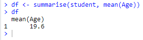
summarise( ) Function

The summarise() function is used to summarize data.

In the example below, we are calculating mean and median for the variable Y2015.

In the following example, we are calculating number of records, mean and median for variables Y2005 and Y2006. The summarise_at function allows us to select multiple variables by their names.

funs( ) has been soft-deprecated (dropped) from dplyr 0.8.0. Instead we should use list . The equivalent code is stated below -

Another way of using it without stating names is through formula instead of function. This is mean = mean function and this is ~mean(.) formula.

You must be wondering about ~ and . symbols. It's a way to pass purrr style anonymous function. See the base R method as compared to purrr style below. Both returns the same output. purrr style provides a shortcut to define anonymous function.

Incase you want to add additional arguments for the functions mean and median (for example na.rm = TRUE ), you can do it like the code below.

We can also use custom functions in the summarise function. In this case, we are computing the number of records, number of missing values, mean and median for variables Y2011 and Y2012. The dot (.) denotes each variables specified in the second argument of the function.

Suppose you want to subtract mean from its original value and then calculate variance of it.

The summarise_if function allows you to summarise conditionally.

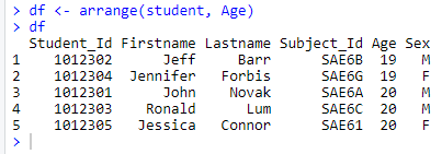
arrange() function

The arrange () function is used to sort data.

The default sorting order of arrange() function is ascending. In this example, we are sorting data by multiple variables.

Suppose you need to sort one variable by descending order and other variable by ascending oder.

Pipe Operator %>%

It is important to understand the pipe (%>%) operator before knowing the other functions of dplyr package. dplyr utilizes pipe operator from another package (magrittr) . It allows you to write sub-queries like we do it in sql.

Note : All the functions in dplyr package can be used without the pipe operator. The question arises "Why to use pipe operator %>%". The answer is it lets to wrap multiple functions together with the use of %>%.

The code below demonstrates the usage of pipe %>% operator. In this example, we are selecting 10 random observations of two variables "Index" "State" from the data frame "mydata".

group_by() function

The group_by() function is used to group data by categorical variable(s).

We are calculating count and mean of variables Y2011 and Y2012 by variable Index.

options(dplyr.summarise.inform=F)

do() function

The do() function is used to compute within groups

Suppose you need to pull top 2 rows from 'A', 'C' and 'I' categories of variable Index.

mutate() function

The mutate() function is used to create new variables.

The following code calculates division of Y2015 by Y2014 and name it "change".

It creates new variables and name them with suffix "_new".

By default, min_rank() assigns 1 to the smallest value and high number to the largest value. In case, you need to assign rank 1 to the largest value of a variable, use min_rank(desc(.))

join() function

The join() function is used to join two datasets.

Combine Data Vertically

The quantile() function is used to determine Nth percentile value. In this example, we are computing percentile values by variable Index.

if() Family of Functions

Let's understand with example. You want to use a variable which is in quotes. In the example below, Species is in quotes. If you use quoted variable directly, it would return zero rows. To make it work, you need to use !! operator which unquotes its argument and gets evaluated immediately in the surrounding context. The final thing we need to do is turn the character string "Species" into Species, a symbol by using sym function.

enquo() is used to quote its argument. Here we are asking user to define variable name without quotes.

In SQL, rank() over(partition by) is used to compute rank by a grouping variable. In dplyr, it can be achieved very easily with a single line of code. See the example below. Here we are calculating rank of variable Y2015 by variable Index.

In dplyr, there are many functions to compute rank other than min_rank( ) . These are dense_rank( ) , row_number( ) , percent_rank() .

across() function

The across( ) function was added starting dplyr version 1.0. It helps analyst to perform same operation on multiple columns. Let's take a sample data.frame mtcars and calculate mean on variables from 'mpg' through 'qsec' by 'carb'.

The code below calculates average on numeric variables. It identifies numeric variables using where() function.

Here we are using two summary statistics - mean and no. of distinct values in two different set of variables.

df %>% mutate(across(c(x, starts_with("y")), mean, na.rm = TRUE)) df %>% mutate(across(everything(), mean, na.rm = TRUE))

There are hundreds of packages that are dependent on this package. The main benefit it offers is to take off fear of R programming and make coding effortless and lower processing time. However, some R programmers prefer data.table package for its speed. I would recommend learn both the packages. The data.table package wins over dplyr in terms of speed if data size greater than 1 GB.

Deepanshu founded ListenData with a simple objective - Make analytics easy to understand and follow. He has over 10 years of experience in data science. During his tenure, he worked with global clients in various domains like Banking, Insurance, Private Equity, Telecom and HR.

Thanks for share, great stuff and examples.

This is the best tutorial out there

excellent! thx Z

Thank you, this is very helpful.

Very helpfull.

Having searched many sites and lectures I am bookmarking your site after looking at this page. Its the simplicity of your presentation. Thanks.

Thank you for stopping by my blog. Glad you found it useful. Cheers!

Thank you, this indeed very helpful and precise. Great Job!

Thank you for your appreciation!

I followed along your script step by step and got a warning message in Example 29 : Multiply all the variables by 1000 as follows: 1: In Ops.factor(c(1L, 1L, 1L, 1L, 2L, 2L, 2L, 3L, 3L, 4L, 5L, 6L, : ‘*’ not meaningful for factors 2: In Ops.factor(1:51, 1000) : ‘*’ not meaningful for factors What did it mean? Could you please give me some explanation. Thanks.

This error says 'multiplying 1000 on factor(string) variables' does not make sense. Run this command - str(mydata[,1:2]) First two variables in the dataframe mydata are strings that are stored as factor variables.

I got it. Thanks. I think I'm ready to go next to your another tutorial - data.table. It's quite interesting to learn R from your blog posts.

Example#22 - gives incorrect number of levels as 0 - fix is below Why doesn't nlevels() work? > summarise_all(dt["Index"], funs(nlevels(.), sum(is.na(.)))) # A tibble: 1 × 2 nlevels sum 1 0 0 =============== The fix is change nlevels() to length(unique(.)) as below summarise_all(dt["Index"], funs(length(unique(.)), sum(is.na(.)))) # A tibble: 1 × 2 length sum 1 19 0

It works fine at my end. Check out the code below - library(dplyr) mydata = read.csv("C:\\Users\\Deepanshu\\Documents\\sampledata.csv") summarise_all(mydata["Index"], funs(nlevels(.), sum(is.na(.))))

Example #21 Alternatively, we can use the following: mydata %>% summarise_if(is.numeric, funs(n(),mean,median))

Thank you for posting alternative method. I have added it to the tutorial. Cheers!

Very helpful tutorial. Thanks!

This is a great tutorial. A doubt that crept to me when I tries to mix multiple functions. Any reason why the following is not working: DF <- mutate_if(mydata, is.numeric & contains('Y2015'), funs('new' = *.100)); but this works: DF <- mutate_if(mydata, is.numeric, funs('new' = *.100)); what if I want to mutate to add only a column for Y2015? Thanks

Great tutorials. Took too much time to found this tutorial.

Wonderfull for a newcomer to R !

Thank you for this great presentation.

Example 39 is wrong.

Try to use below code instead. df = mydata %>% rowwise() %>% mutate(Max= max(Y2012,Y2013,Y2014,Y2015)) %>% select(Y2012:Y2015,Max)

W. r. t. chapter 'SQL-Style CASE WHEN Statement': The workaround .$ is not necessary anymore from dplyr version 0.7.0

Updated. Thanks for pointing it out!

Data manipulation in R using data.table package tutorials is not available. Please fix that

Thanks for highlighting. It's fixed now!

Great tutorial.

Simply superb..Likes your blog a lot..CLEAR CUT EXPLANATION. Super

So many functions explained in such a simple and "easy-to-understand" manner.. Thanks a lot !! :)

Every example is precise, simple and very well explained. Many thanks and congrats!

love the detailed yet simple explanations.

Please help.. mydata %>% filter(Index %in% c("A", "C","I")) %>% group_by(Index) %>%do(head( . , 2)) do(group_by(filter(data,Index%in%c("C","A","I"))),head(.,2)) why am i getting different answers using these codes. Codes are same i guess

é de longe um dos melhores e mais completos tutorias sobre Dplyr. Obrigado!

I am Very thankful to you bro. Bec of u, i have learned dplyr and am using regularly.

sample_n function is not working

What error you are getting? Try this : dplyr::sample_n(iris,3)

Very helpful. Thanks a lot

Really happy to come across this blog...helped me a lot!!

Thank you for stopping by my blog. Cheers!

Any code equivalent for over() (Partition By) function of SQL in DPLYR ?

I added example 49 for the same. Hope it helps!

Sir, powerful package for data manipulations and you made it very easy with your crystal clear explanations with examples.. very helpful stuff made me to learn in two days.. bookmarking your page. Thanks a lot and keep posting for R shiny if possible.. :)

Excellent tutorial , this has helped me a lot

Excellent tutorial and explanations are easy to understand.

The way of flow of explanation and example is appreciable.

How to Use dplyr in R: A Tutorial on Data Manipulation with Examples

Data03.online, tutorial: analyzing star wars character data using tidyverse and dplyr.

In this tutorial, we will explore how to analyze and summarize data from the Star Wars universe using the R programming language. We’ll use the tidyverse package and its dplyr component to perform various data manipulation and analysis tasks on the starwars dataset, which contains information about different characters from the Star Wars series.

Step 1: Loading Libraries and Accessing the Dataset

First, make sure you have the required libraries installed. The tidyverse package provides a collection of packages for data manipulation and visualization. You can install it and load it using the following code:

To access information about the starwars dataset, you can use the ?starwars command. This will display the documentation for the dataset, including details about its columns and data.

Step 2: Filtering and Counting Data

We’ll start by filtering and counting data based on specific criteria using the dplyr functions filter() and count().

In this code, we use the filter() function to extract subsets of data based on specific conditions. We then use nrow() to count the number of rows in the filtered datasets.

Step 3: More Complex Filtering and Counting

Next, we’ll explore more complex filtering and counting using logical operators.

Here, we use the count() function directly, which not only filters the data but also counts the occurrences of different conditions. The | symbol represents logical OR, and the & symbol represents logical AND.

Step 4: Summarizing Data

Moving on, we’ll learn how to summarize data using the summarise() function.

In this code, the summarise() function calculates the mean height of all characters in the starwars dataset. The %>% operator is used to pipe the dataset into the function.

Step 5: Grouping and Summarizing

Now, we’ll explore how to group data by certain categories and then summarize within those groups.

Here, we use the group_by() function to group data by the “species” column. Then, we calculate the mean height within each group using summarise().

Step 6: Calculating Mean and Standard Deviation

Let’s calculate both the mean and standard deviation of mass for each gender.

We use the same approach as before, grouping the data by the “gender” column and then calculating both the mean and standard deviation of mass within each group.

Step 7: Adding a New Column

Finally, we’ll calculate the Body Mass Index (BMI) for each character and add it as a new column in the dataset.

In this code, we use the mutate() function to create a new column named “bmi” by calculating the BMI based on the mass and height columns. The select() function is used to choose only the “mass” and “height” columns from the dataset.

Congratulations! You’ve successfully learned how to manipulate and analyze the Star Wars character data using the tidyverse and dplyr packages in R. These techniques can be applied to various datasets for exploratory data analysis and insights extraction.

To download code visit here: https://www.data03.online/2023/08/how-to-use-dplyr-in-r.html

Data Wrangling with R

Chapter 1 data manipulation using dplyr.

Learning Objectives Select columns in a data frame with the dplyr function select . Select rows in a data frame according to filtering conditions with the dplyr function filter . Direct the output of one dplyr function to the input of another function with the ‘pipe’ operator %>% . Add new columns to a data frame that are functions of existing columns with mutate . Understand the split-apply-combine concept for data analysis. Use summarize , group_by , and count to split a data frame into groups of observations, apply a summary statistics for each group, and then combine the results. Join two tables by a common variable.

Manipulation of data frames is a common task when you start exploring your data in R and dplyr is a package for making tabular data manipulation easier.

Brief recap: Packages in R are sets of additional functions that let you do more stuff. Functions like str() or data.frame() , come built into R; packages give you access to more of them. Before you use a package for the first time you need to install it on your machine, and then you should import it in every subsequent R session when you need it.

If you haven’t, please install the tidyverse package.

tidyverse is an “umbrella-package” that installs a series of packages useful for data analysis which work together well. Some of them are considered core packages (among them tidyr , dplyr , ggplot2 ), because you are likely to use them in almost every analysis. Other packages, like lubridate (to work wiht dates) or haven (for SPSS, Stata, and SAS data) that you are likely to use not for every analysis are also installed.

If you type the following command, it will load the core tidyverse packages.

If you need to use functions from tidyverse packages other than the core packages, you will need to load them separately.

1.1 What is dplyr ?

dplyr is one part of a larger tidyverse that enables you to work with data in tidy data formats. “Tidy datasets are easy to manipulate, model and visualise, and have a specific structure: each variable is a column, each observation is a row, and each type of observational unit is a table.” (From Wickham, H. (2014): Tidy Data https://www.jstatsoft.org/article/view/v059i10 )

The package dplyr provides convenient tools for the most common data manipulation tasks. It is built to work directly with data frames, which is one of the most common data formats to work with.

To learn more about dplyr after the workshop, you may want to check out the handy data transformation with dplyr cheatsheet .

Let’s begin with loading our sample data into a data frame.

We will be working a small subset of the data from the Stanford Open Policing Project . It contains information about traffic stops in the state of Mississippi during January 2013 to mid-July of 2016.

You may have noticed that by using read_csv we have generated an object of class tbl_df , also known as a “tibble”. Tibble’s data structure is very similar to a data frame. For our purposes the relevant differences are that

• it tries to recognize and date types
• the output displays the data type of each column under its name, and
• it only prints the first few rows of data and only as many columns as fit on one screen. If we wanted to print all columns we can use the print command, and set the width parameter to Inf . To print the first 6 rows for example we would do this: print(my_tibble, n=6, width=Inf) .

We are going to learn some of the most common dplyr functions:

• select() : subset columns
• filter() : subset rows on conditions
• mutate() : create new columns by using information from other columns
• group_by() and summarize() : create summary statistics on grouped data
• arrange() : sort results
• count() : count discrete values

1.2 Selecting columns and filtering rows

To select columns of a data frame with dplyr , use select() . The first argument to this function is the data frame ( stops ), and the subsequent arguments are the columns to keep. You may have done something similar in the past using subsetting. select() is essentially doing the same thing as subsetting, using a package (dplyr) instead of R’s base functions.

Alternatively, if you are selecting columns adjacent to each other, you can use a : to select a range of columns, read as “select columns from ___ to ___.”

It is worth knowing that dplyr is backed by another package with a number of helper functions, which provide convenient functions to select columns based on their names. For example:

Other examles are: ends_with() , contains() , last_col() and more. Check out the tidyselect reference for more.

To choose rows based on specific criteria, we can use the filter() function. The argument after the dataframe is the condition we want our resulting data frame to adhere to.

We can also specify multiple conditions within the filter() function. We can combine conditions using either “and” or “or” statements. In an “and” statement, an observation (row) must meet all conditions in order to be included in the resulting dataframe. To form “and” statements within dplyr , we can pass our desired conditions as arguments in the filter() function, separated by commas:

We can also form “and” statements with the & operator instead of commas:

In an “or” statement, observations must meet at least one of the specified conditions. To form “or” statements we use the logical operator for “or”, which is the vertical bar (|):

Here are some other ways to subset rows:

• by row number: slice(stops, 1:3) # rows 1-3
• slice_min(stops, driver_age) # likewise slice_max()
• slice_sample(stops, n = 5) # number of rows to select
• slice_sample(stops, prop = .0001) # fraction of rows to select

To sort rows by variables use the arrange() function:

What if you wanted to filter and select on the same data? For example, lets find drivers over 85 years and only keep the violation and gender columns. There are three ways to do this: use intermediate steps, nested functions, or pipes.

• Intermediate steps:

With intermediate steps, you create a temporary data frame and use that as input to the next function.

This is readable, but can clutter up your workspace with lots of objects that you have to name individually. With multiple steps, that can be hard to keep track of.

• Nested functions

You can also nest functions (i.e. place one function inside of another).

This is handy, but can be difficult to read if too many functions are nested as things are evaluated from the inside out (in this case, filtering, then selecting).

The last option, called “pipes”. Pipes let you take the output of one function and send it directly to the next, which is useful when you need to do many things to the same dataset.

There are now two Pipes in R:

%>% (called magrittr pipe; made available via the magrittr package, installed automatically with dplyr ) or

|> (called native R pipe and it comes preinstalled with R v4.1.0 onwards).

Both the pipes, by and large, function similarly with a few differences (For more information, check: https://www.tidyverse.org/blog/2023/04/base-vs-magrittr-pipe/ ). The choice of which pipe to be used can be changed in the Global settings in R studio and once that is done, you can type the pipe with: Ctrl + Shift + M if you have a PC or Cmd + Shift + M if you have a Mac.

The following example is run using the magrittr pipe, which I will use for the rest of the tutorial.

However, the output will be same with the native pipe so you can feel free to use this pipe as well.

In the above, we use the pipe to send the stops data first through filter() to keep rows where driver_race is Black, then through select() to keep only the officer_id and stop_date columns. Since %>% takes the object on its left and passes it as the first argument to the function on its right, we don’t need to explicitly include it as an argument to the filter() and select() functions anymore.

If we wanted to create a new object with this smaller version of the data, we could do so by assigning it a new name:

Note that the final data frame is the leftmost part of this expression.

Some may find it helpful to read the pipe like the word “then”. For instance, in the above example, we take the dataframe stops , then we filter for rows with driver_age > 85 , then we select columns violation , driver_gender and driver_race . The dplyr functions by themselves are somewhat simple, but by combining them into linear workflows with the pipe, we can accomplish more complex data wrangling operations.

Challenge Using pipes, subset the stops data to include stops in Tunica county only and retain the columns stop_date , driver_age , and violation . Bonus: sort the table by driver age.

1.4 Add new columns

Frequently you’ll want to create new columns based on the values in existing columns or. For this we’ll use mutate() . We can also reassign values to an existing column with that function.

Be aware that new and edited columns will not permanently be added to the existing data frame, munless we explicitly save the output.

So here is an example using the year() function (from the lubridate package, which is part of the tidyverse ) to extract the year of the drivers’ birth:

We can keep adding columns like this, for example, the decade of the birth year:

We are beginning to see the power of piping. Here is a slightly expanded example, where we select the column birth_cohort that we have created and send it to plot:

Figure 1.1: Driver Birth Cohorts

Mutate can also be used in conjunction with logical conditions. For example, we could create a new column, where we assign everyone born after the year 2000 to a group “millenial” and everyone before to “pre-millenial”.

In order to do this we take advantage of the ifelse function:

ifelse(a_logical_condition, if_true_return_this, if_false_return_this)

In conjunction with mutate, this works like this:

More advanced conditional recoding can be done with case_when() .

Challenge Create a new data frame from the stops data that meets the following criteria: contains only the violation column for female drivers of age 50 that were stopped on a Sunday. For this add a new column to your data frame called weekday_of_stop containing the number of the weekday when the stop occurred. Use the wday() function from lubridate (Sunday = 1). Think about how the commands should be ordered to produce this data frame!

1.5 What is split-apply-combine?

Many data analysis tasks can be approached using the split-apply-combine paradigm:

• split the data into groups,
• apply some analysis to each group, and
• combine the results.

Figure 1.2: Split - Apply - Combine

dplyr makes this possible through the use of the group_by() function.

group_by() is often used together with summarize() , which collapses each group into a single-row summary of that group. group_by() takes as arguments the column names that contain the categorical variables for which you want to calculate the summary statistics. So to view the mean age for black and white drivers:

If we wanted to remove the line where driver_race is NA we could insert a filter() in the chain:

Recall that is.na() is a function that determines whether something is an NA . The ! symbol negates the result, so we’re asking for everything that is not an NA .

You can also group by multiple columns:

Note that the output is a “grouped” tibble, grouped by county_name . What it means is that the tibble “remembers” the grouping of the counties, so for any operation you would do after that it will take that grouping into account.

To obtain an “ungrouped” tibble, you can use the ungroup function 1 :

Once the data are grouped, you can also summarize multiple variables at the same time (and not necessarily on the same variable). For instance, we could add a column indicating the standard deviation for the age in each group:

It is sometimes useful to rearrange the result of a query to inspect the values. For that we use arrange() . To sort in descending order, we need to add the desc() function. For instance, we can sort on mean_age to put the groups with the highest mean age first:

1.6 Tallying

When working with data, it is also common to want to know the number of observations found for categorical variables. For this, dplyr provides count() . For example, if we wanted to see how many traffic stops each officer recorded:

Bu default, count will name the column with the counts n . We can change this by explicitly providing a value for the name argument:

We can optionally sort the results in descending order by adding sort=TRUE :

count() calls group_by() transparently before counting the total number of records for each category.

These are equivalent alternatives to the above:

We can also count subgroups within groups:

Challenge Which 5 counties were the ones with the most stops in 2013? Hint: use the year() function from lubridate.

1.7 Joining two tables

It is not uncommon that we have our data spread out in different tables and need to bring those together for analysis. In this example we will combine the numbers of stops for black and white drivers per county together with the numbers of the black and white total population for these counties. The population data are the estimated values of the 5 year average from the 2011-2015 American Community Survey (ACS):

In a first step we count all the stops per county.

We will then pipe this into our next operation where we bring the two tables together. We will use left_join , which returns all rows from the left table, and all columns from the left and the right table. As ID, which uniquely identifies the corresponding records in each table we use the County names.

Now we can, for example calculate the stop rate, i.e. the number of stops per population in each county.

Challenge Which county has the highest and which one the lowest stop rate? Use the snippet from above and pipe into the additional operations to do this.

dplyr join functions are generally equivalent to merge from the R base install, but there are a few advantages .

For all the possible joins see ?dplyr::join

There are currently some experimental features implemented for the summary function tthat might change how grouping and ungrouping are handled in the future ↩︎

Programming with dplyr

Introduction.

Most dplyr verbs use tidy evaluation in some way. Tidy evaluation is a special type of non-standard evaluation used throughout the tidyverse. There are two basic forms found in dplyr:

arrange() , count() , filter() , group_by() , mutate() , and summarise() use data masking so that you can use data variables as if they were variables in the environment (i.e. you write my_variable not df$my_variable ).

across() , relocate() , rename() , select() , and pull() use tidy selection so you can easily choose variables based on their position, name, or type (e.g.  starts_with("x") or is.numeric ).

To determine whether a function argument uses data masking or tidy selection, look at the documentation: in the arguments list, you’ll see <data-masking> or <tidy-select> .

Data masking and tidy selection make interactive data exploration fast and fluid, but they add some new challenges when you attempt to use them indirectly such as in a for loop or a function. This vignette shows you how to overcome those challenges. We’ll first go over the basics of data masking and tidy selection, talk about how to use them indirectly, and then show you a number of recipes to solve common problems.

This vignette will give you the minimum knowledge you need to be an effective programmer with tidy evaluation. If you’d like to learn more about the underlying theory, or precisely how it’s different from non-standard evaluation, we recommend that you read the Metaprogramming chapters in Advanced R .

Data masking

Data masking makes data manipulation faster because it requires less typing. In most (but not all 1 ) base R functions you need to refer to variables with $ , leading to code that repeats the name of the data frame many times:

The dplyr equivalent of this code is more concise because data masking allows you to need to type starwars once:

Data- and env-variables

The key idea behind data masking is that it blurs the line between the two different meanings of the word “variable”:

env-variables are “programming” variables that live in an environment. They are usually created with <- .

data-variables are “statistical” variables that live in a data frame. They usually come from data files (e.g.  .csv , .xls ), or are created manipulating existing variables.

To make those definitions a little more concrete, take this piece of code:

It creates a env-variable, df , that contains two data-variables, x and y . Then it extracts the data-variable x out of the env-variable df using $ .

I think this blurring of the meaning of “variable” is a really nice feature for interactive data analysis because it allows you to refer to data-vars as is, without any prefix. And this seems to be fairly intuitive since many newer R users will attempt to write diamonds[x == 0 | y == 0, ] .

Unfortunately, this benefit does not come for free. When you start to program with these tools, you’re going to have to grapple with the distinction. This will be hard because you’ve never had to think about it before, so it’ll take a while for your brain to learn these new concepts and categories. However, once you’ve teased apart the idea of “variable” into data-variable and env-variable, I think you’ll find it fairly straightforward to use.

Indirection

The main challenge of programming with functions that use data masking arises when you introduce some indirection, i.e. when you want to get the data-variable from an env-variable instead of directly typing the data-variable’s name. There are two main cases:

When you have the data-variable in a function argument (i.e. an env-variable that holds a promise 2 ), you need to embrace the argument by surrounding it in doubled braces, like filter(df, {{ var }}) .

The following function uses embracing to create a wrapper around summarise() that computes the minimum and maximum values of a variable, as well as the number of observations that were summarised:

When you have an env-variable that is a character vector, you need to index into the .data pronoun with [[ , like summarise(df, mean = mean(.data[[var]])) .

The following example uses .data to count the number of unique values in each variable of mtcars :

Note that .data is not a data frame; it’s a special construct, a pronoun, that allows you to access the current variables either directly, with .data$x or indirectly with .data[[var]] . Don’t expect other functions to work with it.

Name injection

Many data masking functions also use dynamic dots, which gives you another useful feature: generating names programmatically by using := instead of = . There are two basics forms, as illustrated below with tibble() :

If you have the name in an env-variable, you can use glue syntax to interpolate in:

If the name should be derived from a data-variable in an argument, you can use embracing syntax:

Learn more in ?rlang::`dyn-dots` .

Tidy selection

Data masking makes it easy to compute on values within a dataset. Tidy selection is a complementary tool that makes it easy to work with the columns of a dataset.

The tidyselect DSL

Underneath all functions that use tidy selection is the tidyselect package. It provides a miniature domain specific language that makes it easy to select columns by name, position, or type. For example:

select(df, 1) selects the first column; select(df, last_col()) selects the last column.

select(df, c(a, b, c)) selects columns a , b , and c .

select(df, starts_with("a")) selects all columns whose name starts with “a”; select(df, ends_with("z")) selects all columns whose name ends with “z”.

select(df, where(is.numeric)) selects all numeric columns.

You can see more details in ?dplyr_tidy_select .

As with data masking, tidy selection makes a common task easier at the cost of making a less common task harder. When you want to use tidy select indirectly with the column specification stored in an intermediate variable, you’ll need to learn some new tools. Again, there are two forms of indirection:

When you have the data-variable in an env-variable that is a function argument, you use the same technique as data masking: you embrace the argument by surrounding it in doubled braces.

The following function summarises a data frame by computing the mean of all variables selected by the user:

When you have an env-variable that is a character vector, you need to use all_of() or any_of() depending on whether you want the function to error if a variable is not found.

The following code uses all_of() to select all of the variables found in a character vector; then ! plus all_of() to select all of the variables not found in a character vector:

The following examples solve a grab bag of common problems. We show you the minimum amount of code so that you can get the basic idea; most real problems will require more code or combining multiple techniques.

User-supplied data

If you check the documentation, you’ll see that .data never uses data masking or tidy select. That means you don’t need to do anything special in your function:

One or more user-supplied expressions

If you want the user to supply an expression that’s passed onto an argument which uses data masking or tidy select, embrace the argument:

This generalises in a straightforward way if you want to use one user-supplied expression in multiple places:

If you want the user to provide multiple expressions, embrace each of them:

If you want to use the name of a variable in the output, you can embrace the variable name on the left-hand side of := with {{ :

Any number of user-supplied expressions

If you want to take an arbitrary number of user supplied expressions, use ... . This is most often useful when you want to give the user full control over a single part of the pipeline, like a group_by() or a mutate() .

When you use ... in this way, make sure that any other arguments start with . to reduce the chances of argument clashes; see https://design.tidyverse.org/dots-prefix.html for more details.

Creating multiple columns

Sometimes it can be useful for a single expression to return multiple columns. You can do this by returning an unnamed data frame:

This sort of function is useful inside summarise() and mutate() which allow you to add multiple columns by returning a data frame:

Notice that we set .unpack = TRUE inside across() . This tells across() to unpack the data frame returned by quantile_df() into its respective columns, combining the column names of the original columns ( x and y ) with the column names returned from the function ( val and quant ).

If your function returns multiple rows per group, then you’ll need to switch from summarise() to reframe() . summarise() is restricted to returning 1 row summaries per group, but reframe() lifts this restriction:

Transforming user-supplied variables

If you want the user to provide a set of data-variables that are then transformed, use across() and pick() :

You can use this same idea for multiple sets of input data-variables:

Use the .names argument to across() to control the names of the output.

Loop over multiple variables

If you have a character vector of variable names, and want to operate on them with a for loop, index into the special .data pronoun:

This same technique works with for loop alternatives like the base R apply() family and the purrr map() family:

(Note that the x in .data[[x]] is always treated as an env-variable; it will never come from the data.)

Use a variable from an Shiny input

Many Shiny input controls return character vectors, so you can use the same approach as above: .data[[input$var]] .

See https://mastering-shiny.org/action-tidy.html for more details and case studies.

Introduction to R

Chapter 4 data manipulation with dplyr.

dplyr is a package that makes data manipulation easy. It consists of five main verbs:

summarise()

Other useful functions such as glimpse()

4.1 Excercise

• Import the customer data into R using read_csv("path") , save it to a data.frame
• Use glimpse() on it

4.2 filter()

filter() is a function that let’s you filter out rows that meet certain conditions.

We can also use text:

And combine them:

We can also filter out every row that meets a condition in a vector, for instance:

4.2.1 Operators

In R, as in any programming languange, there are a number of logical and relational operators.

In R these are:

4.3 We also have operators for checking if something is TRUE

• Instead of writing x == TRUE you should write isTRUE(x) and !isTRUE(x) if you want to check if something is FALSE .

4.3.1 Use filter to find…

How many customers had a data-volume over 1000 in february 2019?

How many customers have been members longer than 2005

How many customers have a data-volume over 2000 in february and have a calculated revenue larger than 500 per month?

How many customers have a subscription with “Rörlig pris”?

Are there any customers that are missing an ID? I.e. is NA .

4.3.2 stringr

• When working filter() it is common that we want to filter out certains parts of a string
• stringr is a great package for manipulating strings in R
• Usually it’s functions starts with str_... , such as str_detect() .

Here are some useful functions:

Or str_replace()

Or str_remove()

4.3.3 stringr in filter()

We can use stringr in filter() :

• Specific string manipulation

For example:

4.5 Excercise 2

• How many customers have a subscription with “Fast pris”?
• How many customers have a subscription that is not “Bredband”?

4.6 arrange()

arrange() is a verb for sorting data.frames.

If you instead want to sort in descending order you can write like this:

4.6.0.1 Excercise 3

• Which customer has been “active” longest? What is the date?
• Which customer is most newly active?

4.7 select()

select() is a verb for selecting columns in a data.frame.

You can choose columns by their name:

You can also choose columns based on their numerical order

You can select all the columns from column_a to column_d with : :

4.7.1 Help functions

When you do data science you often want to move columns for different reasons. Not seldom you want to put one column first and the rest after. For this you can use the help function everything() :

Apart from eveything() there are a number of other help functions:

starts_with(“asd”)

ends_with(“air”)

contains(“flyg”)

matches(“asd”)

num_range(“flyg”, 1:10) matches flyg1, flyg2 … flyg10

You can use these in the same way as everything() .

4.8 rename()

To rename a variable you use rename(data, new_variable = old_variable)

4.9 Excercise 4

Choose all columns that contain ”nm"

Choose the column for customer ID and all columns that starts with ”tr_tot"

Rename ”pc_priceplan_nm" to ”price_plan"

4.10 mutate()

• mutate() is a verb for manipulating and creating new columns

Below we create a new column with the mean of departure delay.

You can also use with simple mathematical operators mutate() :

There is a variant of mutate mutate() called transmute() that will return only the column that you have maniuplated.

In combination with mutate() you can use a variety of functions, some example of useful functions inside mutate is:

rank(), min_rank(), dense_rank(), percent_rank() to rank

log(), log10() to take the log of a variable

cumsum(), cummean() for cummulative stats

row_number() if you need to create rownumbers

lead() and lag()

For example we can lag departure delay and save it in a new variable.

4.10.1 if_else()

• A common task in Excel or any other programming languange is to compose if else -statements.
• The best way to do this in R is with the function if_else()

If you want to make multiple if else -statements, instead of making multiple if else -statements you can use the case_when() function:

4.11 Excercise 5

Create a new variable that is the mean of the last 3 months of data consumption

Create a variable that takes the logarithm of your previously created column

Create a new variable that indicates if the priceplan is “Bredband” or not.

Create a new variable that groups priceplan in “Fast pris”, “Rörligt pris”, “Bredband” and “Annan” for everything that is not in any of the previous.

• Dates a information about time that we commonly use in analytics.
• The easiest way to manipulate dates in R is with the package lubridate .

In order to get todays date you can use the function Sys.Date() (that is built into R).

Say that you want to find the month, week or year of a date.

The package lubridate contains useful functions for this, such as year() , month() and week .

In general you should define your date before passing it to a lubridate-function. In other words, you can’t just use a string (even though that sometimes work).

You can define you with with as.Date() , where you also can specify the format of the date.

This is especially useful if your date is written in a non-standard way.

Other functions that are useful in lubridate are days_in_month :

And floor_date() if you, for example, want to find the first date in a month or a week,.

4.13 Excercise 6

• Create a varible for month lubridate::month(x) of customer activation
• Create a new varibale for year of customer activation
• Create a new variable with the number of days in the month of activation

4.14 summarise()

summarise() is a verb for summarizing data (you can also spell i summarize() ).

4.14.1 group_by()

Below we create a new grouped data set grouped on carrier och dest .

Every summarisation or mutation done on this new data-set will be done group wise.

4.15 Excercise 7

• What is the sum data volume during the last month? What’s the mean and median and what are the max and min values? You can use max() and min() to calculate maximum and minimum-values.

4.15.1 More expressions

You can combine dplyr -verbs

However, the more verbs you combine the harder it will be to read:

4.15.1.1 %>% “the pipe”

• %>% from the magrittr -package. %>% is called “the pipe” and is pronounced “and then”.

4.16 Excercise 8

Use %>% and answer the following questions:

Which CPE type is most common?

Which priceplan has the highest mean data volume (for febraury 2019)?

Calculate the mean of data volume for the year that the customer was created. Which year has the highest mean?

To join data frames is an essential part of data manipulation, to do that we use dplyr ’s different join functions:

• left_join()
• right_join()
• full_join()
• inner_join()
• semi_join()
• anti_join()

4.18 Joins som venn

4.19 Excercise 9

• Left join your data with tele2-kunder-transaktioner.csv on custid .

4.20 Tidy data

• tidy data is when every observation is a row and every variable is a column.

4.21 Untidy data

We want to gather the columns

• spread() does the opposite.

4.22 Excercise 10

In your data set you have 12 columns for data volume consumption per month, tr_tot_data_vol_all_netw_1:tr_tot_data_vol_all_netw_12

Every column represent a month and you want to calculate the mean of data volume consumption over time.

The columns represent a month

The first column tr_tot_data_vol_all_netw_1 is the latest month, i.e. “2019-04-30”

Create a vector with all the month dates corresponding to the columns.

R function called seq()

Rename every column by it’s date.

• Fill in the sort(decreasing = ) to TRUE
• Gather the data into two new columns called data_month and data_volume
• Turn data_month into a date-column
• Calculate the mean value per priceplan and month

Execute the code to visualize:

<iframe src=“plotly_ex.html” width = “900px”, height = “600px” frameBorder=“0”>

R news and tutorials contributed by hundreds of R bloggers

Complete dplyr tutorial for data analytics and data manipulation in r.

Posted on January 14, 2016 by DataCamp Blog in R bloggers | 0 Comments

[social4i size="small" align="align-left"] --> [This article was first published on DataCamp Blog , and kindly contributed to R-bloggers ]. (You can report issue about the content on this page here ) Want to share your content on R-bloggers? click here if you have a blog, or here if you don't.

A video of Garrett Grolemund explaining the dplyr package in the DataCamp course

The dplyr tutorial

The DataCamp interactive learning environment

To leave a comment for the author, please follow the link and comment on their blog: DataCamp Blog . R-bloggers.com offers daily e-mail updates about R news and tutorials about learning R and many other topics. Click here if you're looking to post or find an R/data-science job . Want to share your content on R-bloggers? click here if you have a blog, or here if you don't.

Copyright © 2022 | MH Corporate basic by MH Themes

Never miss an update! Subscribe to R-bloggers to receive e-mails with the latest R posts. (You will not see this message again.)

Numpy Ninja

Career-centric company, just  for women.

• Jun 27, 2020

Data Manipulation using DPLYR : Part 1

In this blog, you will learn how to easily perform data manipulation using R software . We’ll use mainly the popular dplyr R package, which contains important R functions to carry out easily your data manipulation. The dplyr package(written by Hadley Wickham) provides us with several functions that facilitate the manipulation of data frames in R. Some of the most useful include:

1. The select Function: facilitates the selection of records (rows)

2. The filter Function: facilitates the selection of variables (columns)

3. The arrange Function: facilitates the ordering of records

4. The mutate Function: facilitates the creation of new variables

5. The rename Function: facilitates the renaming of variables

6. The summarize Function: facilitate the summarization of variables

At the end of this blog, you will be familiar with data manipulation tools and approaches that will allow you to efficiently manipulate data.

What is Data Manipulation ?

If you are still confused with this ‘term’, let me explain it to you. Data Manipulation is a loosely used term with ‘Data Exploration’. It involves ‘manipulating’ data using available set of variables. This is done to enhance accuracy and precision associated with data.

Actually, the data collection process can have many loopholes. There are various uncontrollable factors which lead to inaccuracy in data such as mental situation of respondents, personal biases, difference / error in readings of machines etc. To mitigate these inaccuracies, data manipulation is done to increase the possible (highest) accuracy in data. At times, this stage is also known as data wrangling or data cleaning.

Required R package

First, you need to install the dplyr package and load the dplyr library then after you can able to perform the following data manipulation functions.

Demo Datasets

1. The select Function

The select function allows us to choose the columns to keep within a dataset. This can be done by simply specifying the column names (or numbers) to retain. You can perform data manipulations on either dataframe or CSV file.

Now, you can choose any number of columns using select function. Here, columns 1 to 3 and 5 columns are chosen using both column name and number which shows in below snippet:

You can use negatives to select columns to drop:

There are a number of additional supporting functions you can use in order to identify columns to select or omit, such as “contains”, “starts_with” and “ends_with” :

2. The filter Function

The filter function allows us to choose specific rows from a data frame. You achieve this by specifying a logical statement:

3. The arrange Function

The arrange function allows us to sort the data on 1 or more variables. You provide values which specify the variables by which to sort in ascending order:

You can use the desc function to specify that a variable be sorted in descending order:

4. The mutate Function

You can create new variables within a data frame using the mutate function:

Tip : the ifelse function can be used for conditional logic when creating variables.

5. The rename Function

The rename function provides a neat and highly readable way to rename columns:

You can also rename multiple variables at once:

Tip : The new name is on the left and the old name is on the right.

6. The summarize Function

Often when analyzing a dataset we want to calculate summary statistics; You can do this with the summarize function, in conjunction with several basic summary functions:

Standard summaries such as mean, median, min, max etc.

Additional functions provided by dplyr: n, n_distinct

Sums of logicals, such as sum(x > 10)

If you have missing data we can add an option na.rm = TRUE that will find the summary value even if there are missing values.

Notice that the default column names are equal to the call that was made. You can replace these by specifying a new column name:

In this blog on data manipulation in R, we discussed the functions of manipulation of data in R. The dplyr package provides us with several functions that facilitate the manipulation of data (e.g., select, filter, arrange, mutate, summarize, rename).

When calling the functions:

The first argument is the input data frame,

The remaining arguments describe what to do to the data frame

The function outputs a data frame.

Recent Posts

Tableau for data Analytics

Beginner Friendly Java String Interview Questions

Hello Everyone! Welcome to the second section of the Java Strings blog. Here are some interesting coding questions that has been solved with different methods and approaches. “Better late than never!”

Data Chaining and Data Driven Testing in API Testing using Postman

Navigation Menu

Instantly share code, notes, and snippets.

d-smith / tidy-scripts.R

• Download ZIP
• Star 2 You must be signed in to star a gist
• Fork 5 You must be signed in to fork a gist
• Embed Embed this gist in your website.
• Share Copy sharable link for this gist.
• Clone via HTTPS Clone using the web URL.
• Learn more about clone URLs
• Save d-smith/04e755d7345505191ff5 to your computer and use it in GitHub Desktop.

Masdarul commented Apr 20, 2024

stuck 55%, in 3 kali

Sorry, something went wrong.

Data transformation with dplyr :: Cheatsheet

Download PDF

Translations (PDF)

dplyr functions work with pipes and expect tidy data . In tidy data:

• Each variable is in its own column
• Each observation , or case , is in its own row
• pipes x |> f(y) becomes f(x,y)

Summarize Cases

Apply summary functions to columns to create a new table of summary statistics. Summary functions take vectors as input and return one value back (see Summary Functions).

summarize(.data, ...) : Compute table of summaries.

count(.data, ..., wt = NULL, sort = FLASE, name = NULL) : Count number of rows in each group defined by the variables in ... . Also tally() , add_count() , and add_tally() .

Group Cases

Use group_by(.data, ..., .add = FALSE, .drop = TRUE) to created a “grouped” copy of a table grouped by columns in ... . dplyr functions will manipulate each “group” separately and combine the results.

Use rowwise(.data, ...) to group data into individual rows. dplyr functions will compute results for each row. Also apply functions to list-columns. See tidyr cheatsheet for list-column workflow.

ungroup(x, ...) : Returns ungrouped copy of table.

Manipulate Cases

Extract cases.

Row functions return a subset of rows as a new table.

filter(.data, ..., .preserve = FALSE) : Extract rows that meet logical criteria.

distinct(.data, ..., .keep_all = FALSE) : Remove rows with duplicate values.

slice(.data, ...,, .preserve = FALSE) : Select rows by position.

slice_sample(.data, ..., n, prop, weight_by = NULL, replace = FALSE) : Randomly select rows. Use n to select a number of rows and prop to select a fraction of rows.

slice_min(.data, order_by, ..., n, prop, with_ties = TRUE) and slice_max() : Select rows with the lowest and highest values.

slice_head(.data, ..., n, prop) and slice_tail() : Select the first or last rows.

Logical and boolean operations to use with filter()

• See ?base::Logic and ?Comparison for help.

Arrange cases

arrange(.data, ..., .by_group = FALSE) : Order rows by values of a column or columns (low to high), use with desc() to order from high to low.

add_row(.data, ..., .before = NULL, .after = NULL) : Add one or more rows to a table.

Manipulate Variables

Extract variables.

Column functions return a set of columns as a new vector or table.

pull(.data, var = -1, name = NULL, ...) : Extract column values as a vector, by name or index.

select(.data, ...) : Extract columns as a table.

relocate(.data, ..., .before = NULL, .after = NULL) : Move columns to new position.

Use these helpers with select() and across()

• contains(match)
• num_range(prefix, range)
• : , e.g., mpg:cyl
• ends_with(match)
• all_of(x) or any_of(x, ..., vars)
• ! , e.g., !gear
• starts_with(match)
• matches(match)
• everything()

Manipulate Multiple Variables at Once

across(.cols, .fun, ..., .name = NULL) : summarize or mutate multiple columns in the same way.

c_across(.cols) : Compute across columns in row-wise data.

Make New Variables

Apply vectorized functions to columns. Vectorized functions take vectors as input and return vectors of the same length as output (see Vectorized Functions).

mutate(.data, ..., .keep = "all", .before = NULL, .after = NULL) : Compute new column(s). Also add_column() .

rename(.data, ...) : Rename columns. Use rename_with() to rename with a function.

Vectorized Functions

To use with mutate().

mutate() applies vectorized functions to columns to create new columns. Vectorized functions take vectors as input and return vectors of the same length as output.

• dplyr::lag() : offset elements by 1
• dplyr::lead() : offset elements by -1

Cumulative Aggregate

• dplyr::cumall() : cumulative all()
• dply::cumany() : cumulative any()
• cummax() : cumulative max()
• dplyr::cummean() : cumulative mean()
• cummin() : cumulative min()
• cumprod() : cumulative prod()
• cumsum() : cumulative sum()
• dplyr::cume_dist() : proportion of all values <=
• dplyr::dense_rank() : rank with ties = min, no gaps
• dplyr::min_rank() : rank with ties = min
• dplyr::ntile() : bins into n bins
• dplyr::percent_rank() : min_rank() scaled to [0,1]
• dplyr::row_number() : rank with ties = “first”
• + , - , / , ^ , %/% , %% : arithmetic ops
• log() , log2() , log10() : logs
• < , <= , > , >= , != , == : logical comparisons
• dplyr::between() : x >= left & x <= right
• dplyr::near() : safe == for floating point numbers

Miscellaneous

dplyr::case_when() : multi-case if_else()

dplyr::coalesce() : first non-NA values by element across a set of vectors

dplyr::if_else() : element-wise if() + else()

dplyr::na_if() : replace specific values with NA

pmax() : element-wise max()

pmin() : element-wise min()

Summary Functions

To use with summarize().

summarize() applies summary functions to columns to create a new table. Summary functions take vectors as input and return single values as output.

• dplyr::n() : number of values/rows
• dplyr::n_distinct() : # of uniques
• sum(!is.na()) : # of non-NAs
• mean() : mean, also mean(!is.na())
• median() : median
• mean() : proportion of TRUEs
• sum() : # of TRUEs
• dplyr::first() : first value
• dplyr::last() : last value
• dplyr::nth() : value in the nth location of vector
• quantile() : nth quantile
• min() : minimum value
• max() : maximum value
• IQR() : Inter-Quartile Range
• mad() : median absolute deviation
• sd() : standard deviation
• var() : variance

Tidy data does not use rownames, which store a variable outside of the columns. To work with the rownames, first move them into a column.

tibble::rownames_to_column() : Move row names into col.

tibble::columns_to_rownames() : Move col into row names.

Also tibble::has_rownames() and tibble::remove_rownames() .

Combine Tables

Combine variables.

• bind_cols(..., .name_repair) : Returns tables placed side by side as a single table. Column lengths must be equal. Columns will NOT be matched by id (to do that look at Relational Data below), so be sure to check that both tables are ordered the way you want before binding.

Combine Cases

• bind_rows(..., .id = NULL) : Returns tables one on top of the other as a single table. Set .id to a column name to add a column of the original table names.

Relational Data

Use a “Mutating Join” to join one table to columns from another, matching values with the rows that the correspond to. Each join retains a different combination of values from the tables.

• left_join(x, y, by = NULL, copy = FALSE, suffix = c(".x", ".y"), ..., keep = FALSE, na_matches = "na") : Join matching values from y to x .
• right_join(x, y, by = NULL, copy = FALSE, suffix = c(".x", ".y"), ..., keep = FALSE, na_matches = "na") : Join matching values from x to y .
• inner_join(x, y, by = NULL, copy = FALSE, suffix = c(".x", ".y"), ..., keep = FALSE, na_matches = "na") : Join data. retain only rows with matches.
• full_join(x, y, by = NULL, copy = FALSE, suffix = c(".x", ".y"), ..., keep = FALSE, na_matches = "na") : Join data. Retain all values, all rows.

Use a “Filtering Join” to filter one table against the rows of another.

• semi_join(x, y, by = NULL, copy = FALSE, ..., na_matches = "na") : Return rows of x that have a match in y . Use to see what will be included in a join.
• anti_join(x, y, by = NULL, copy = FALSE, ..., na_matches = "na") : Return rows of x that do not have a match in y . Use to see what will not be included in a join.

Use a “Nest Join” to inner join one table to another into a nested data frame.

• nest_join(x, y, by = NULL, copy = FALSE, keep = FALSE, name = NULL, ...) : Join data, nesting matches from y in a single new data frame column.

Column Matching for Joins

Use by = join_by(col1, col2, …) to specify one or more common columns to match on.

Use a logical statement, by = join_by(col1 == col2) , to match on columns that have different names in each table.

Use suffix to specify the suffix to give to unmatched columns that have the same name in both tables.

Set Operations

• intersect(x, y, ...) : Rows that appear in both x and y .
• setdiff(x, y, ...) : Rows that appear in x but not y .
• union(x, y, ...) : Rows that appear in x or y, duplicates removed. union_all() retains duplicates.
• Use setequal() to test whether two data sets contain the exact same rows (in any order).

CC BY SA Posit Software, PBC • [email protected] • posit.co

Learn more at dplyr.tidyverse.org .

Updated: 2023-07.

Secure Your Spot in Our R Programming Online Course - Register Now (Click for More Info)

The Ultimate Course to Quickly Master Data Manipulation in R Using dplyr & the tidyverse

All you need to know to handle your data like an expert without wasting your time with too much unnecessary talk.

This R course shows you exactly how to get your data ready for use, step-by-step.

• Even if… you’ve struggled with R programming in the past.
• Even if… you’re new to R programming.
• Even if… you’ve understood Base R, but don’t know where to start with the tidyverse.
• Even if… you’ve thought to yourself “the dplyr syntax is too complicated for me”.

What You Get

Learn data manipulation with our interactive course ! Enjoy self-paced videos, refine your newly acquired skills by engaging in quizzes that range from simple to advanced, and ask your questions directly to the Statistics Globe team and other learners in our exclusive LinkedIn chat.

We invite you to join us in weekly public discussions spanning 8 weeks starting from November 27, 2023, where we’ll elaborate on the video lessons, dive deeper into recent exercises and real-world projects, and navigate through all sorts of questions together.

Please note: While we have a structured 8-weeks plan, your journey through the course is entirely in your hands . Whether you take several months or just a weekend to go through the materials is completely up to you.

Upon completion of the course, you will retain access to all videos, learning materials, and resources for future reference. The group chat will remain active, enabling future exchanges and networking with fellow participants. Additionally, you will receive a certificate verifying your attendance in the course.

Here are some more details on the structure of the course!

A Peek Inside the Course

Dive into the exciting world of data manipulation with our interactive online course on R , dplyr , and the tidyverse !

Through easy-to-follow modules, you’ll gain practical skills to manage, analyze, and visualize data, boosting your career prospects in the thriving field of data science.

Ideal for R programming beginners as well as advanced users that want to make the switch from Base R coding to the tidyverse approach .

With this course, you’ll not only gain a better understanding of data manipulation and dplyr; You’ll also boost your general skills in R programming.

Here’s the table of contents of the entire course! You will receive video lessons, simple to advanced exercises, as well as additional learning materials on each of those topics.

Table of Contents

• Course Structure & About the Instructor
• dplyr & the tidyverse Overview
• Installing & Loading dplyr
• tibble vs. data.frame
• The Pipe Operator
• Creating tibbles
• Working with Columns
• Working with Rows [ Course Preview ]
• Importing & Exporting Data Using dplyr & readr
• Replacing Values
• Handling Missing Values
• Binding Rows & Columns
• Grouping Data
• Joining Data Sets
• Reshaping Data Using dplyr & tidyr
• Data Visualization Using dplyr & ggplot2
• Handling Character Strings Using dplyr & stringr
• Handling Dates & Times Using dplyr & lubridate
• Advanced Data Manipulation Project – Pt. 1
• Advanced Data Manipulation Project – Pt. 2
• Summary & Further Resources

Love It or Return It: 30 Days Money-Back Guarantee

Your purchase is absolutely risk-free with our straightforward money-back guarantee! We are confident that our course will not disappoint you. However, if you don’t like what you see, you can get a 100% refund up to 30 days after the course has started.

Meet Your Instructor: Joachim Schork

Hey, I’m Joachim Schork and back in the days, when I started my journey as a programmer and statistician, mastering R programming felt like an impossible challenge to me.

After finishing my bachelor’s degree in Educational Science, I decided to focus more on programming and statistical methodology, but when I started my master’s in survey statistics, I felt hopeless . Do you know that moment when you scream at your PC screen after several hours of unsuccessful coding attempts?

Since the start of my educational journey, I have used online resources to complement the university’s official learning materials. This has helped me a lot, but at the same time I felt like I was often spending too much time on a video or blog article because many of these resources don’t get straight to the point.

This was one of the reasons why I founded Statistics Globe more than five years ago. Meanwhile, I had completed my master’s degree, got my first job at a national statistical institute in Europe, and was even rewarded with an EMOS certificate that approves special knowledge in the field of official statistics. I had gained extensive knowledge in the area that I wanted to pass on.

However, I didn’t want to create endless tutorials that didn’t fulfill the need of its users. Instead, I created straightforward content designed to guide users to solutions for their problems as quickly as possible.

Now, five years later, Statistics Globe has gained:

20 million clicks on the website

3 million clicks on YouTube videos

50 thousand followers across Social Media platforms

• 23,763 YouTube Subscribers
• 18,616 Facebook Group Members
• 5,663 LinkedIn Followers
• 5,505 X/Twitter Followers

This is such an incredible success, and I’m so thankful to everybody who participated in this journey! And please don’t get me wrong: I don’t want to brag about these numbers, but I think they can show you that my content works.

With this video course, it’s the first time I’ve combined all of this experience and knowledge into a single resource on data manipulation using tidyverse’s fabulous but often misused dplyr package.

By the way, this is the very first time that I charge anything for content on Statistics Globe. All other content remains free.

However, the conception and implementation of this course requires my full-time work for several months, and all other Statistics Globe team members are also involved. I hope you understand that it is not possible to run such a video course without compensation.

This course is such a big milestone for me, and I’m so excited. I love exchanging with other data enthusiasts, and I am looking forward to our discussions in our exclusive group chat. I promise that I will invest all my passion and a lot of time into this course to make it an outstanding experience to all of us.

I’m not the only one who will support you in this course, though! The entire Statistics Globe team is ready to answer your questions , no matter if you have problems understanding any of the lessons or exercises, or if you have technical issues with the R software, the example data, or the add-on packages that we’ll use in the course.

In case you have further questions or anything else you would like to talk about, feel free to email me to [email protected] , write me via the contact form , or send me a message via my Social Media channels.

I’ve created a video that explains the structure and the content of the course in more detail.

By clicking this button, you’ll be added to a waiting list to receive future updates about the course. I’d be honored to welcome you to the next course. 🙂

Subscribe to the Statistics Globe Newsletter

Get regular updates on the latest tutorials, offers & news at Statistics Globe. I hate spam & you may opt out anytime: Privacy Policy .

22 Comments . Leave new

I am eagerly awaiting to join and learn from you.

Thank you very much for your registration to the course. I’ll let you know more details via email soon.

Regards, Joachim

I will be happy to participate to this R programming courses.

Hi Jonathan,

Thank you for your registration, it’s great to have you in the course. You will receive an email shortly with further details.

Hi Mustafa,

glad you like the idea, we are all pretty excited.

R for Windows problem

Thanks for your comment. Could you specify your question in some more detail?

Hi Joachim,

I am from a clinical research background with no previous knowledge of any programming knowledge, will it be ok for me to go for this course

Thank you for your message and your interest in the course.

Yes, that would be possible. We start the course with some R programming and tidyverse basics, and then we slowly move on to more advanced topics.

There are, by the way, already some participants with a clinical background. 🙂

Please let me know in case you have further questions.

When do you plan to start the registrations? As I am working, I would have to plan my reskilling by specifying the learning dates to my management. Alternatively, is it possible to enroll for the previous course?

Regards, Abhishek

Hi Abhishek,

Happy New Year!

Thank you for your interest in the course. Currently, we are working on another course that will start soon ( more info ). I’m not sure when this course will take place the next time. Unfortunately, it’s not possible to register to the running course at this point, since it will be finished soon.

I’ll inform you as early as possible when I know the next starting date for this course. Make sure to join the waiting list, I’ll send all the information there.

Best regards, Joachim

Je veux un lien pour télécharger le logiciel R

Hello Amira,

You can find the instructions on the posit’s website . You should download both Rstudio and R.

Best, Cansu

Good luck 🙂

Thanks for the kind words, Jimmy! 🙂

I completed the Data Manipulation in R Using dplyr & the tidyverse course. I would highly recommend. I had some experience in R but was self taught so this course was really helpful in giving me some more structure to my data analysis and fill in the gaps of my R knowledge. I would especially recommend to any PhD students researcher wanting to get started in R! The course load is also very manageable around full-time work.

Thank you so much for this wonderful feedback! It’s really great to hear that you enjoyed the course, and that you would recommend it to others! 🙂

All the best, Joachim

I highly recommend everyone who needs statistics to join this course.

Thank you so much for the kind comment and your recommendation. It’s great to hear that you liked the course!

when you will be starting again for this course ?

Hey Mohammed,

Thank you for your interest in the course! It has not yet been decided when the course will be held again. I recommend joining the waiting list (see button above) to be informed about the next course.

Leave a Reply Cancel reply

Your email address will not be published. Required fields are marked *

Post Comment

dplyr tutorial

Dplyr is one of the main packages in the tidyverse universe, and one of the most used packages in R. Without a doubt, dplyr is a very powerful package, since allows you to manipulate data very easily, and it enables you to work with other languages and frameworks, such as SQL, Spark o R’s data.table.

Besides, as it is part of the tidyverse universe, it is very easy to use dplyr with other packages within tidyverse, such as ggplot , which allows, for example, to make very cool graphics in a simple way and without having to create any intermediate objects.

As you can see, dplyr is very powerful. However, do you know exactly how it works, all the features it offers, and why it is so powerful? Well, in this tutorial I will explain everything you need to know about dplyr. And you’ll even have exercises to practice. There is much to learn, so set’s get to it!

Installation and pipe operator

The first thing we will have to do is install dplyr. To do this, you simply have to run the following code:

dplyr includes the %>% operator, called pipe, which is very useful and applicable to the entire tidyverse ecosystem. This operator allows you to concatenate functions in such a way that the data is passed from one function to another without having to assign it to any variable.

For example, suppose we want to rank cars that have more than 100 horsepower by their gas mileage (mpg variable) in descending order. Let’s see how we would do it without using the pipe operator.

Now, let’s see how we would do it with the pipe operator:

As we can see, the result is exactly the same, but by using the pipe we have avoided having to create intermediate objects, so if we wanted to change our transformation it would be very simple. Also, the code is much cleaner if we use the pipe operator.

Now that you know what the pipe operator is, let’s continue with the dplyr tutorial, gradually seeing what are the main functions of dplyr focused on different transformations.

Main functions of dplyr

Basically, dplyr has 5 different groups of functions: summary, grouping, selection/filter, manipulation, and combination functions.

Although the value of dplyr lies in being able to combine all these functions to be able to manipulate data in a simple and clean way, in order to do that it is essential to first know the main functions that the package offers.

So, let’s go step by step knowing each of the functions of each group. Let’s get to it!

dplyr grouping functions

The grouping functions allow grouping the data in such a way that we can apply certain functions for each of the groups. There are basically two types of functions: group_by and ungroup .

group_by function

The group_by function allows grouping the data into different groups based on one or more variables of our dataframe. When a dataframe is grouped, it is still a single dataframe, but the operations we do will apply to each of the groups. This is why the group_by function is rarely used alone, but will most likely be used with other dplyr functions, such as summarize or mutate .

Likewise, it is important to emphasize that the most common is to group based on one or more variables in text or categorical format since it rarely makes sense that several numerical observations have the same (although it may be the case).

In our case, we are going to use the gapminder dataset, which contains data on life expectancy, population, and GDP per Capita of different countries for different years. This is the dataset:

Let’s imagine that we want to obtain the average life expectancy for each continent for each year so that we can visualize how life expectancy has evolved by continent.

To do this, we will group the data by continent and year and use the summarize function (which I will explain later) to obtain the average life expectancy.

As we can see, with only 3 lines of code we have managed to make a very interesting summary of the data. Thus, almost all the functions that we are going to learn in this dplyr tutorial can be applied with grouped data.

Exercise of the group_by function

To check that you have understood, I propose the following exercise: calculate the average life expectancy worldwide, for each year.

Ungroup function

Sometimes, we do a grouping to obtain grouped data (the total sum of the variable, for example), but we do not want to continue performing operations with the grouped data. In that case, we will have to ungroup the data, and this can be done with the ungroup function.

For example, suppose that for a specific year (say 1952) we want to show a graph in which we compare each of the countries with the average life expectancy of their continent. To do this, you would simply have to:

• Filter the data by the year we want.
• Group the data by continent.
• Calculate the average life expectancy of the continent.
• Ungroup the data.

As we can see, all the countries of the same continent have the same mean_lifeExp , which makes sense, because the average life expectancy of a continent is the same for all the countries of the continent.

And with this, you already know the grouping functions. As you can see, grouping functions are usually used with other functions, so let’s continue with this dplyr tutorial and learn new dplyr functions!

dplyr filter and selection functions

Select () function.

The select function is very simple, it allows you to indicate the columns that you want to select or stop using. Usually, when you manipulate data you create quite some auxiliary variables to check something or to calculate new fields. These are variables that generally you won’t want in the final dataset. For this reason, this function is usually used to only keep the variables you want.

Another use case is when the dataset includes more variables than you are going to use for analysis. In those cases, keeping only the variables that interest you from the beginning will allow you to:

• Make the code faster.
• Make the results more easily interpretable, since there will be no noisy variables.

To select some variables, you just have to pass the name of the columns to the function:

Likewise, the select function also allows you to drop variables too, that is, to deselect one or more columns. To do this, simply pass the symbol – in front of the variable. Example:

Exercise select function

To practice the dplyr select function, I propose the following exercise: from the gapminder dataframe, choose the variables continent, year and lifeExp. First, you must do it by selecting the variables that interest you.

Now, get the same result, but in a different way, using dplyr’s select function:

Filter function

The filter function allows you to filter the data for one or more conditions that we pass to it. For example, as we have done in the previous example, we can filter the data to keep only cars with more than 100 horsepower (hp).

When it comes to numeric variables, there are six filters that we can apply: greater than (>), less than (<), equal to (==), different than (! =), greater than or equal to (> =) and less or equal to (<=).

In addition, for numeric variables, the filter function also allows you to filter the variables that are text or factor. In this case, there are three options that we can apply: equal to (==), different from (! =), it is included in (% in% c ()), it is not included in (! Value% in% c () ).

Let’s see an example with the Species variable of the iris dataset, which is a factor that has 3 values:

In addition, we can combine several filters, in such a way that we can filter, at the same time, by several variables, each one with its condition. In these cases there are two options: that both options must be met, in which case the filters are joined by the symbol & or that either of the two options must be satisfied, in which case the | symbol is used.

As you can see, the filter function is very intuitive and very powerful, since it allows you to filter information in a much more intuitive and clear way than R’s default filters.

Filter function exercises

To practice the filter function, I am going to ask you to keep the observations from the gapminder dataset that: they are from Africa, that the year is 2007 and that the life expectancy is greater than 60 years.

distinct() function

The distinct function is very simple since it allows us to eliminate duplicated data from our dataset. This is something that does not make sense in a clean dataset, but it becomes handy when we have to clean and transform the data.

To do this, we are going to create a new dataset, named iris_duplicate , which will basically contains the duplicate iris dataset. So, we will see how this function works:

As we can see, the iris dataset has 150 observations, but one of them must be duplicated (or the values coincide), since if we apply the distinct function we will be left with 149 observations.

Also, even though the iris_duplicate dataset has 300 observations, after applying the distinct function we are left with the 149 values that are unique.

slice () function

The slice function allows you to keep the data of the positions that we say. That is if we run slice (1) we will keep the first value, and if we run slice(1:20) , we will keep the first 20 values:

Although it seems like a very silly function, the slice function is very useful especially when applied with the group_by function, since it will allow us to obtain the number of values ​​that we want for each of the groups. In fact, this is what I used to create a bar chart race in the post about how to create animations with R .

Likewise, there are other slice functions that allow you to perform the same task, but with some modification. For example, the slice_min and slice_max functions allow you to get the rows with the minimum or maximum value of a variable.

This, combined with the group_by function, is very powerful, since in two lines we are able to obtain the observations with maximum values ​​for each group. With Gapminder, for example, we can obtain the country with the highest life expectancy (LifeExp) by continent and year.

On the other hand, the slice_sample function allows you to obtain a random amount of data, which can be very useful, for example, to split the data between train, test, and validation, in order to train a machine-learning model.

Finally, the slice_head and slice_tail functions allow you to obtain the amount of data you want starting at the top (head) or bottom (tail) and respecting the current order of the data.

Now that you know how it works, let’s see how to use them in practice.

Exercises slice function

Using the Gapminder dataset and some function of the slice family, find the countries with the highest life expectancy each year.

Now, find the 5 countries with the highest life expectancy of each year.

Arrange function

The arrange function allows you to sort the data based on one or more variables, both ascending and descending. By default, the data will be sorted in ascending order, to indicate that it is sorted in descending order, we will have to wrap the variable with the desc function.

For example, suppose we want to sort the cars according to their consumption (mpg):

As we can see, the cars are ordered, but there are cases in which the mpg value coincides, as in the case of the Honda and Lotus (30.4) or the Datsu and Mercedes (22.8).

In those cases, the function will sort according to the position they were in the dataframe. However, we can indicate that it orders them by another variable, such as the horses (hp) in descending order as well:

As we can see, in this case both the Lotus and the Mercedes appear ahead of the Honda and the Datsu, since, with equal consumption, they have more horses.

Arrange function exercise

Let’s put everything we’ve seen about dplyr’s arrange function into practice. To do this, I ask you to order the gapminder dataset by year (newest first), continent (from Z to A) and by life expectancy (from lowest to highest).

And with this very simple (and practical) function you have already seen the most important filtering functions within dplyr. As you can see, a simple but very interesting and practical function.

However, dplyr hides much more, so let’s continue with the tutorial, in this case with summary functions.

Summary functions

The summary functions are usually used, almost always, after a grouping function ( group_by ), since this allows to obtain metrics for each one of the groups in a very simple way.

summarize function

The summarize (or summarize ) function allows obtaining data from each of the groups, such as the maximum, minimum, mean, standard deviation, number of observations, etc.

To do this, you simply have to:

• Indicate the name of the new column that will be created.
• Pass the function and the variable that will be used to obtain said column.

For example, we could get the mean, maximum, and mean life expectancy of the entire dataset. We can obtain this in the following way:

In this case, since the data is not grouped, the calculations are performed on the entire dataset. However, as I mentioned previously, the most common is to use the summarize function together with the group_by function, in such a way that the calculations are performed for each of the groups.

For example, let’s say we want to get the mean, minimum, and maximum of life expectancy, but instead of for the entire dataset, we want to see it for each year. This could be obtained as follows:

Exercise summarize function

Let’s put the summarize function into practice! Using this function and some other function we have seen so far, calculate the maximum, minimum and mean of the population and life expectancy for each continent and year. The variables should be called lifeExp_min, lifeExp_max, lifeExp_mean and pop_min, pop_max and pop_mean, in that order.

As you can see, the summarize function is very very powerful. Above all, if it is combined with the next function that we are going to see, let’s continue with our complete dplyr tutorial!

Across function

It could be the case that we want to calculate a series of functions (minimum, maximum, mean and number of cases, for example) to several columns. With what we have seen so far, one option would be to indicate one by one each of the operations (maximum, minimum, etc.) for each column. However, this does not seem very efficient …

In those cases, a better option is to use the across function. The across function allows us to apply the functions that we indicate to the columns that we indicate. Although the end result is the same, using the across function is much more optimal, since (1) it will take less time, (2) you are less likely to make mistakes and also (3) the code will remain a lot cleaner.

Let’s imagine that we want to calculate the maximum, minimum and mean for life expectancy and population. Without using the across function we would do it as follows:

As you can see, the above code works, but it is quite cumbersome. Now, let’s try doing it with the across function:

As we can see, we obtain the same result in much fewer lines of code, it is much easier to read and modify.

In fact, with the across function we can pass conditionals, such as, for example, that the column is numeric, or factor. Let’s see an example, obtaining the mode of the categorical variables and the mean of the numerical variables:

Note: to use fashion, I have used the function indicated in this post.

Exercise across function

As you can see, the across function is very useful, and it would have saved us a lot of time in the previous exercise. That is why, I ask you again to calculate the minimum, maximum, and average life expectancy and the population of each continent in each year, but this time using the across function.

count function

Finally, another very recurring question is to obtain the number of cases/observations in each group. Although this could be obtained with the summarize function, another faster way to obtain it is with the count function.

Let’s look at an example assuming that we want to obtain the number of countries for which we have data for each of the years. Using the summarize function, it would be done as follows:

However, another faster option is to use the count function directly:

As we can see, we save a few lines, again, making our code more easily understandable.

Have a look at the summary functions! Let’s continue with this dplyr tutorial looking at the manipulation functions.

dplyr data manipulation functions

The manipulation functions allow you to modify the current columns, either by creating new ones or renaming the current columns.

Within the data manipulation functions we find the functions: mutate , transmute , add_column , rename . Also, although they are not from the dplyr package, but from the tidyr package, I will comment on the pivot_wider and pivot_longer functions, since which are also very frequent in dplyr pipes.

mutate function

The mutate function allows you to create new columns, which will be the result of applying a function. Therefore, within the mutate function, we must always have two elements: the name of the new column and the function that will result in the values ​​of the column.

For example, we can use the mutate function to check if the name of the passenger on the Titanic included Mr .:

As we can see, the mutate function is very simple, but at the same time very useful, since it avoids having to make many assignments and / or corrections, which later is to know if they have been made or no.

In this sense, a function widely used together with mutate is the case_when function, which allows you to create conditionals in a very simple way.

For example, we could create a new variable called Gender that returns Man if the name includes Mr. & nbsp; or Master, Woman if it includes Ms., Mrs. & nbsp; or Miss, for example.

In addition, it may be the case that a name does not fall into any of the previous categories. In this case we could indicate that it is an NA, for example.

Doing this with the case_when function is very simple:

Mutate exercises

Using the titanic dataset, create a new Boolean column, called adult, which returns TRUE if the person is of legal age or FALSE if he is not.

As we can see, making modifications with mutate is very simple, it’s faster than doing a normal assignment and makes the code more understandable.

However, there will be times when we just want to create a couple of new variables and forget about the rest. Although we could do that with a mutate function followed by a select , an easier way is to use the function transmute .

Transmute function

The transmute function allows us to create new variables and get rid of the rest of the variables. For example, imagine that we want to analyze the relationship between the variable sex and the name of the person, to check how many times the default variable Gender is correct (that is, we want to analyze the internal consistency of the data).

For this, we could use, for example, a mutate function followed by a filter :

But, another simpler option and do it all within the same function, using transmute .

rename function

Another very common case is when we want to change the name of a column. With what we’ve seen so far, this could be done with the mutate function. However, a simpler and clearer way is to do it with the rename function.

Modifying the name with mutate would be done like this:

Whereas with the rename function, the process is somewhat simpler:

pivot_longer and pivot_wider functions

Although these two functions are not from the dplyr library, but from the tidyr library, they are very useful and, generally, widely used in dplyr pipes.

The idea of ​​these functions is simple: go from having several variables in a column to having one variable per column or, vice versa, going from one variable per column to a column with several variables.

In the first case (from several variables in one column to one column per variable), we will use the pivot_wider function.

In this function you simply have to indicate:

• The columns that should not be modified.
• Which column will create the columns (in our case, the year).
• What variable will be used to fill the columns new columns (in our case, lifeExp).

This function is useful, especially when there is redundancy in the data, as in this case it happens with the year column.

On the contrary, we can go from wide data to narrower ones, making several variables are included within the same column.

We can achieve this with the pivot_longer function, in which we only have to choose the columns to pivot, the name of the column where the names of the variables will go and the name of the column where it will go the value:

Given the data manipulation functions, we would only have one family of functions left: the data combination functions.

Data combination functions

The data combination functions serve precisely for that: to combine information from two dataframes or tibbles. These combinations can be of two types:

• Horizontal join: when a dataframe adds more columns than already exist. Within these functions we would find the bind_cols function, the joins: left_join , right_join , inner_join and full_join , as well as filter functions based on join, such as semi_join and anti_join .
• Vertical join: when a dataframe includes more rows. Within this type of functions we would find: bind_rows , union , intersect , setdiff and setequal .

So, let’s see how these functions work!

bind_rows and bind_cols function

The bind_rows and bind_cols functions are similar to the rbind and cbind functions, although they have some of the same features main differences are:

• bind_rows directly manages the lists, whereas rbind you must use the do.call function.
• bind_rows is much more efficient than rbind , although bind_cols is not more efficient than cbind .
• bind_rows handles mismatched columns, including NAs, while rbind will fail.

As an example, we can compare the efficiency of cbind with bind_cols :

And we can do the same with the rbind and bind_rows functions:

As we can see, when it comes to binding rows, dplyr’s bind_rows is much more efficient. Although this is not noticeable with little data, it is something that becomes important when we start working with larger datasets.

Now, let’s see how join functions work.

Join functions: left_join, right_join, inner_join, full_join, semi_join and anti_join

Join functions allow you to join data horizontally. Each of the functions will return a different result. For example:

• left_join : returns all cells in the table on the left, even if they do not match the table on the right.
• right_join : returns the data from the table on the right, even if it does not match the data from the table on the left.
• inner_join : only returns the data that matches in both tables.
• semi_join : returns the data from X (X only) that match the key of Y.
• anti_join: displays the X data (X only) that has no match with the Y key.
• full_join: returns the X and Y data, but does not match.

A good way to look at it is through examples. To do this, we are going to see a typical case of ecommer analysis, since the information is usually stored for each purchase in a table.

If we wanted to get the customers and their order data, we should simply do a left_join :

In this case, we will have 38 columns, (14 from clients, 25 from orders – the join column). In addition, even though there are only 21 customers, we have 22 rows, since the same customer may have made more than one purchase.

Likewise, we could obtain the order data only from those customers who have made purchases, for which we will use the inner_join :

It could also be the case that we want the data of the customers who have placed orders, but we are not interested in including the order data, but we simply want to know which customers they are. To do this, we can use the semi_join function.

As we can see, there are only 8 customers at our customer table who have placed orders. Or what is the same, there are 9 people at the customer table who have not placed orders. So if we wanted to identify these users, we could use the anti_join function:

Indeed, the function returns those 11 customers from the customer table who have not placed orders.

You may not see big differences between using semi_join and / or anti_join compared to the filter function. Although it is true that for these cases we could obtain the same result with the filter function, the filter function only works for those cases in which there is a single key, while The semi_join and anti_join functions serve regardless of the number of keys in the table.

Join exercises

Enrich the calls that have a client, using the inner_join function.

Now, do the same process, but using the left_join function. Important: the left_join may return data that you are not interested in, so you will have to use another function that we have learned to solve it.

With this, in our complete guide to dplyr we have already seen all the families of functions that the package has. Now let’s see some practical cases where they can be interesting.

Practical examples of the dplyr library

Visualizing gapminder data with dplyr and ggplot.

A classic dplyr use case is to create a cool visualization from a dataframe with ggplot . And, the dplyr functions that we have learned in the tutorial together with the pivot_wider and pivot_longer functions offer practically everything you need to be able to make all kinds of visualizations.

For example, in this case, starting from the original gapminder dataset, we will create a dplyr pipe that allows us to visualize the average, maximum and minimum evolution for each of the continents and each of the variables we have.

To do this, we will use the group_by , summarize and across functions to calculate the maximum, minimum and mean for each of the continents in every year.

Once this is done, we will transform the data in long format with pivot_longer . Thus, we can use the mutate function to have the function that has been used and the value of the function separately.

Once we have this, we will pivot the data again, this time in wide-format using pivot_wider , so that we have the data ready to be painted with ggplot2 .

As a result, we see a very interesting and useful graph that allows us to see curious things, such as the growth of the population in Asia in recent years, the convergence of life expectancy and the increase in the differences in terms of GDP per Capita in Europe, the general increase in life expectancy on all continents.

And all this has been obtained using only 4 dplyr functions, 2 tidyr functions and the ggplot2 library, all in a fairly simple and friendly code.

Manipulating stream data with dplyr

A typical case of dplyr pipes is when the observations refer to different actions within a flow, such as the positions of a taxi or the pages visited by users on the web.

Although there are no typical datasets for this type of data, we will use the gapminder dataset to show how it would be used in this type of case. To do this, we will make a Sankey visualization that shows the evolution of the countries with the highest GDP per Capita for different years, the data being the difference with respect to the next country.

For this, we will again use the packages, dplyr , ggplot2 and alluvial , which allows us to make sankey graphics in ggplot2 . We are going to create a Sankey diagram that allows us to see how the deviation from the mean has evolved in terms of GDP per Capita of the ten countries with the highest GDP per Capita each year.

To do this, we are simply going to group the data by year and sort it by GDP per Capita in descending order. In this way, with mutate we can: (1) obtain the position of each country for that year, (2), for each country obtain the deviation with respect to the average GDP per capita of that year.

As we can see, with a few dplyr functions we have been able to transform the data to have it in such a way that I could easily create the Sankey graph.

Conclusions from the dplyr tutorial

If dplyr is one of the most used R packages, it is because it is a very simple library to understand and with which you get a very understandable and very efficient code.

Also, being part of one of the tidyverse world packages, its integration with other packages of the “universe”, such as ggplot2 or tidyr makes it very practical, being able to create complex and visually stunning visualizations without the need to save any intermediate objects.

So, I hope this complete tutorial on dplyr has helped you get to know the package better. Also, don’t forget to take a look at the post about how to create animations in R with gganimate , which complements this post very well. If you want to be aware of the posts I publish, I recommend that you subscribe to my blog. And, if you liked it and can afford it, I would appreciate it if you could contribute a donation to allow me to continue creating more content like this. In any case, see you in the next post!

Table of Contents

Don't miss a post.

If you like what you read ... subscribe to keep up to date with the content I upload. You will be the first to know!

I've read and I accepted the privacy policy .

Successful subscription!

Ander Fernández Jauregui | Legal Notice

• Privacy Overview
• Strictly Necessary Cookies
• Cookies de terceros
• Cookie Policy

This website uses cookies so that we can provide you with the best user experience possible. Cookie information is stored in your browser and performs functions such as recognising you when you return to our website and helping our team to understand which sections of the website you find most interesting and useful.

Strictly Necessary Cookie should be enabled at all times so that we can save your preferences for cookie settings.

If you disable this cookie, we will not be able to save your preferences. This means that every time you visit this website you will need to enable or disable cookies again.

Esta web utiliza Google Analytics para recopilar información anónima tal como el número de visitantes del sitio, o las páginas más populares.

Dejar esta cookie activa nos permite mejorar nuestra web.

Please enable Strictly Necessary Cookies first so that we can save your preferences!

More information about our Cookie Policy

Data Science with R

Chapter 4 data manipulation using dplyr and tidyr, learning objectives.

• Describe the purpose of the dplyr and the tidyr packages written by (Wickham, François, et al. 2020 ) and (Wickham and Henry 2020 ) , respectively.
• Select certain columns in a data frame with the dplyr function select .
• Select certain rows in a data frame according to filtering conditions with the dplyr function filter .
• Link the output of one dplyr function to the input of another function with the ‘pipe’ operator %>% .
• Add new columns to a data frame that are functions of existing columns with mutate .
• Use the split-apply-combine concept for data analysis.
• Use summarize , group_by , and count to split a data frame into groups of observations, apply summary statistics for each group, and then combine the results.
• Describe the concept of a wide and a long table format and for which purpose those formats are useful.
• Describe what key-value pairs are.
• Reshape a data frame from long to wide format and back with the pivot_wider and pivot_longer commands from the tidyr package.
• Export a data frame to a .csv file.

Bracket subsetting is handy, but it can be cumbersome and difficult to read, especially for complicated operations. Enter dplyr . dplyr is a package for making tabular data manipulation easier. It pairs nicely with tidyr which enables you to swiftly convert between different data formats for plotting and analysis.

Packages in R are basically sets of additional functions that let you do more stuff. The functions we’ve been using so far, like str() or data.frame() , come built into R ; packages give you access to more of them. Before you use a package for the first time you need to install it on your machine, and then you should import it in every subsequent R session when you need it. You should already have installed the tidyverse package written by (Wickham 2019 ) . This is an “umbrella-package” that installs several packages useful for data analysis which work together well such as tidyr , dplyr , ggplot2 , tibble , etc.

The tidyverse package tries to address 3 common issues that arise when doing data analysis with some of the functions that come with R:

• The results from a base R function sometimes depend on the type of data.
• Using R expressions in a non standard way, which can be confusing for new learners.
• Hidden arguments, having default operations that new learners are not aware of.

We have seen in our previous lesson that when building or importing a data frame, the columns that contain characters (i.e., text) are coerced (=converted) into the factor data type. We had to set stringsAsFactors to FALSE to avoid this hidden argument to convert our data type.

This time we will use the tidyverse package to read the data and avoid having to set stringsAsFactors to FALSE

If we haven’t already done so, we can type install.packages("tidyverse") straight into the console. In fact, it’s better to write this in the console than in our script for any package, as there’s no need to re-install packages every time we run the script.

Then, to load the package type:

4.1 What are dplyr and tidyr ?

The package dplyr provides easy tools for the most common data manipulation tasks. It is built to work directly with data frames, with many common tasks optimized by being written in a compiled language (C++). An additional feature is the ability to work directly with data stored in an external database. The benefits of doing this are that the data can be managed natively in a relational database, queries can be conducted on that database, and only the results of the query are returned.

This addresses a common problem with R in that all operations are conducted in-memory and thus the amount of data you can work with is limited by available memory. The database connections essentially remove that limitation in that you can connect to a database of many hundreds of GB, conduct queries on it directly, and pull back into R only what you need for analysis.

The package tidyr addresses the common problem of wanting to reshape your data for plotting and use by different R functions. Sometimes we want data sets where we have one row per measurement. Sometimes we want a data frame where each measurement type has its own column, and rows are instead more aggregated groups - like plots or aquaria. Moving back and forth between these formats is non-trivial, and tidyr gives you tools for this and more sophisticated data manipulation.

To learn more about dplyr and tidyr after the workshop, you may want to check out this handy data transformation with dplyr cheatsheet and this one about tidyr .

We’ll read in our data using the read_csv() function, from the tidyverse package readr , instead of using the base R read.csv() function.

You will see the message Parsed with column specification , followed by each column name and its data type. When you execute read_csv on a data file, it looks through the first 1000 rows of each column and guesses the data type for each column as it reads it into R. For example, in this dataset, read_csv reads weight as col_double (a numeric data type), and species as col_character . You have the option to specify the data type for a column manually by using the col_types argument in read_csv .

Notice that the class of the data is now tbl

This is referred to as a “tibble”. Tibbles tweak some of the behaviors of the data frame objects we introduced in the previous episode. The data structure is very similar to a data frame. For our purposes the only differences are that:

• In addition to displaying the data type of each column under its name, it only prints the first few rows of data and only as many columns as fit on one screen.
• Columns of class character are never converted into factors.

We’re going to learn some of the most common dplyr functions:

• select() : subset columns
• filter() : subset rows on conditions
• mutate() : create new columns by using information from other columns
• group_by() and summarize() : create summary statistics on grouped data
• arrange() : sort results
• count() : count discrete values

4.2 Selecting columns and filtering rows

To select columns of a data frame, use select() . The first argument to this function is the data frame ( surveys ), and the subsequent arguments are the columns to keep.

To select all columns except certain ones, put a “-” in front of the variable to exclude it.

This will select all the variables in surveys except record_id and species_id .

To choose rows based on a specific criterion, use filter() :

What if you want to select and filter at the same time? There are three ways to do this: use intermediate steps, nested functions, or pipes.

With intermediate steps, you create a temporary data frame and use that as input to the next function, like this:

This is readable, but can clutter up your workspace with lots of objects that you have to name individually. With multiple steps, that can be hard to keep track of.

You can also nest functions (i.e. one function inside of another), like this:

This is handy, but can be difficult to read if too many functions are nested, as R evaluates the expression from the inside out (in this case, filtering, then selecting).

The last option, pipes , are a recent addition to R. Pipes let you take the output of one function and send it directly to the next, which is useful when you need to do many things to the same dataset. Pipes in R look like %>% and are made available via the magrittr package written by (Bache and Wickham 2014 ) , which is installed automatically with dplyr . If you use RStudio, you can type the pipe with Ctrl + Shift + M if you have a PC or Cmd + Shift + M if you have a Mac.

In the above code, we use the pipe to send the surveys dataset first through filter() to keep rows where weight is less than 5, then through select() to keep only the species_id , sex , and weight columns. Since %>% takes the object on its left and passes it as the first argument to the function on its right, we don’t need to explicitly include the data frame as an argument to the filter() and select() functions any more.

Some may find it helpful to read the pipe like the word “then”. For instance, in the above example, we took the data frame surveys , then we filter ed for rows with weight < 5 , then we select ed columns species_id , sex , and weight . The dplyr functions by themselves are somewhat simple, but by combining them into linear workflows with the pipe, we can accomplish more complex manipulations of data frames.

If we want to create a new object with this smaller version of the data, we can assign it a new name:

Note that the final data frame is the leftmost part of this expression.

• Using pipes, subset the surveys data to include animals collected before 1995 and retain only the columns year , sex , and weight .

Frequently you’ll want to create new columns based on the values in existing columns, for example to do unit conversions, or to find the ratio of values in two columns. For this we’ll use mutate() .

To create a new column of weight in kg:

You can also create a second new column based on the first new column within the same call of mutate() :

If this runs off your screen and you just want to see the first few rows, you can use a pipe to view the head() of the data. (Pipes work with non- dplyr functions, too, as long as the dplyr or magrittr package is loaded).

The first few rows of the output are full of NA s, so if we wanted to remove those we could insert a filter() in the chain:

is.na() is a function that determines whether something is an NA . The ! symbol negates the result, so we’re asking for every row where weight is not an NA .

Create a new data frame from the surveys data that meets the following criteria: contains only the species_id column and a new column called hindfoot_cm containing the hindfoot_length values converted to centimeters. In this hindfoot_cm column, there are no NA s and all values are less than 3.

Hint : think about how the commands should be ordered to produce this data frame!

4.5 Split-apply-combine data analysis and the summarize() function

Many data analysis tasks can be approached using the split-apply-combine paradigm: split the data into groups, apply some analysis to each group, and then combine the results. dplyr makes this very easy through the use of the group_by() function.

4.5.1 The summarize() function

group_by() is often used together with summarize() , which collapses each group into a single-row summary of that group. group_by() takes as arguments the column names that contain the categorical variables for which you want to calculate the summary statistics. So to compute the mean weight by sex :

You may also have noticed that the output from these calls doesn’t run off the screen anymore. It’s one of the advantages of tbl_df over data frame.

You can also group by multiple columns:

When grouping both by sex and species_id , the last few rows are for animals that escaped before their sex and body weights could be determined. You may notice that the last column does not contain NA but NaN (which refers to “Not a Number”). To avoid this, we can remove the missing values for weight before we attempt to calculate the summary statistics on weight. Because the missing values are removed first, we can omit na.rm = TRUE when computing the mean:

Here, again, the output from these calls doesn’t run off the screen anymore. If you want to display more data, you can use the print() function at the end of your chain with the argument n specifying the number of rows to display:

Once the data are grouped, you can also summarize multiple variables at the same time (and not necessarily on the same variable). For instance, we could add a column indicating the minimum weight for each species for each sex:

It is sometimes useful to rearrange the result of a query to inspect the values. For instance, we can sort on min_weight to put the lighter species first:

To sort in descending order, we need to add the desc() function. If we want to sort the results by decreasing order of mean weight:

4.5.2 Counting

When working with data, we often want to know the number of observations found for each factor or combination of factors. For this task, dplyr provides count() . For example, if we wanted to count the number of rows of data for each sex, we would do:

The same type of traditional cross-tabulation is accomplished in base R with table() and xtabs() .

The count() function is shorthand for something we’ve already seen: grouping by a variable, and summarizing it by counting the number of observations in that group. In other words, surveys %>% count() is equivalent to:

For convenience, count() provides the sort argument:

The previous example shows the use of count() to enumerate the number of rows/observations for one factor (i.e., sex ). If we wanted to count a combination of factors , such as sex and species , we would specify the first and the second factor as the arguments of count() :

With the above code, we can proceed with arrange() to sort the table according to a number of criteria so that we have a better comparison. For instance, we might want to arrange the table above in (i) an alphabetical order of the levels of the species and (ii) in descending order of the count:

From the table above, we may learn that, for instance, there are 75 observations of the albigula species that are not specified for its sex (i.e. NA ).

How many animals were caught in each plot_type ?

Use group_by() and summarize() to find the mean, min, and max hindfoot length for each species (using species_id ). Also add the number of observations (hint: see ?n ).

What was the heaviest animal measured in each year? Return the columns year , genus , species_id , and weight .

4.6 Reshaping with pivot_longer() and pivot_wider()

The spreadsheet lesson discusses how to structure data to satisfy the four rules defining a tidy dataset. The four rules defining a tidy dataset are:

• Each variable has its own column
• Each observation has its own row
• Each value must have its own cell
• Each type of observational unit forms a table

Figure 4.1: Following three rules makes a dataset tidy: variables are in columns, observations are in rows, and values are in cells.

Note: The Tidy data subsection material comes from R for Data Science with slight modifications.

You can represent the same underlying data in multiple ways. The example below shows the same data organized in four different ways. Each dataset shows the same values of four variables country , year , population , and cases , but each dataset organizes the values in a different way.

These are all representations of the same underlying data, but they are not equally easy to use. One dataset, the tidy dataset ( table1 ), will be much easier to work with inside the tidyverse .

4.6.1 Longer — Using pivot_longer()

A common problem is a dataset where some of the column names are not names of variables, but values of a variable. Take table4a ; the column names 1999 and 2000 represent values of the year variable. The values in the 1999 and 2000 columns represent values of the cases variable, and each row represents two observations, not one.

To tidy a dataset like this, we need to gather/pivot the offending columns into a new pair of variables. To describe that operation we need three parameters:

The set of columns whose names are values, not variables. In this example, those are the columns 1999 and 2000 .

The name of the variable to move the column names to. Here it is year .

The name of the variable to move the column values to. Here it is cases .

Together those parameters generate the call to pivot_longer() :

The columns to gather are specified with dplyr::select() style notation. Here there are only two columns, so we list them individually. Note that “1999” and “2000” are non-syntactic names (because they don’t start with a letter) so we have to surround them in backticks. In the final result, the pivoted columns are dropped, and we get new year and cases columns. Otherwise, the relationships between the original variables are preserved. Visually, this is shown in Figure 4.2 .

Figure 4.2: Pivoting table4 into a longer, tidy form.

pivot_longer() makes datasets longer by increasing the number of rows and decreasing the number of columns.

4.6.2 Wider — Using pivot_wider()

pivot_wider() is the opposite of pivot_longer() . You use it when an observation is scattered across multiple rows. For example, take table2 : an observation is a country in a year, but each observation is spread across two rows.

To tidy this up, we first analyse the representation in similar way to pivot_longer() . This time, however, we only need two parameters:

The column to take variable names from. Here it’s type .

The column that contains values from multiple variables. Here it’s count .

Once we’ve figured that out, we can use pivot_wider() , as shown programmatically below, and visually in Figure 4.3 .

Figure 4.3: Spreading table2 makes it tidy

As you might have guessed from their names, pivot_wider() and pivot_longer() are complements. pivot_longer() makes wide tables narrower and longer; pivot_wider() makes long tables shorter and wider.

Here we examine the fourth rule: Each type of observational unit forms a table.

In surveys , the rows of surveys contain the values of variables associated with each record (the unit), values such as the weight or sex of each animal associated with each record. What if instead of comparing records, we wanted to compare the different mean weight of each genus between plots ( plot_id )? (Ignoring plot_type for simplicity).

We’d need to create a new table where each row (the unit) is comprised of values of variables associated with each plot ( plot_id ). In practical terms this means the values in genus would become the names of column variables and the cells would contain the values of the mean weight observed on each plot ( plot_id ).

Having created a new table, it is therefore straightforward to explore the relationship between the weight of different genera within, and between, the plots. The key point here is that we are still following a tidy data structure, but we have reshaped the data according to the observations of interest: average genus weight per plot ( plot_id ) instead of recordings per date.

The opposite transformation would be to transform column names into values of a variable.

We can do both of these transformations with two tidyr functions, pivot_wider() and pivot_longer() .

4.6.3 Wider

pivot_wider() takes three principal arguments:

• the column to take variable names_from whose values will become new column names.
• the column that contains values_from multiple variables whose values will fill the new column variables.

Further arguments include fill which, if set, fills in missing values with the value provided.

Let’s use pivot_wider() to transform surveys to find the mean weight of each genus in each plot over the entire survey period. We use filter() , group_by() and summarise() or equivalently summarize() to filter our observations and variables of interest, and to create a new variable for the mean_weight .

This yields surveys_gw where the observations for each plot are spread across multiple rows, 196 observations of 3 variables. Using pivot_wider() with names_from genus and values_from mean_weight this becomes 24 observations of 11 variables, one row for each plot.

We could now plot comparisons between the weight of genera in different plots.

4.6.4 Longer

The opposing situation could occur if we had been provided with data in the form of surveys_spread , where the genus names are column names, but we wish to treat them as values of a genus variable instead.

In this situation we are pivoting the column names and turning them into a pair of new variables. One variable represents the names_to , and the other variable contains the values_to .

pivot_longer() takes four principal arguments:

the cols is the columns in the survey_spread data frame you either want or do not want to “tidy”. Observe how we set this to -plot_id indicating we to not want to tidy the plot_id variable of surveys_spread and rather only the variables Baiomys ,…, Spermophillus . Since plot_id appears in surveys_spread we do not put quotation marks around it.

the names_to here corresponds to the name of the variable in the new “tidy” data frame that will contain the column names of the original data. Observe how we set names_to = "genus" . In the resulting surveys_gather , the column genus contains the ten types of genus. Since genus is a variable name that doesn’t appear in surveys_spread , we use quotation marks around it. You will receive an error if you just use names_to = genus .

the values_to column here is the name of the variable in the new “tidy” data frame that will contain the values of the original data. Observe how we set values_to = "mean_weight" since each of the numeric values in each of the genus columns of surveys_spread data corresponds to a value of mean_weight . Note again that mean_weight does not appear as a variable in surveys_spread so it again needs quotation marks around if for the values_to argument.

To recreate surveys_gw from surveys_spread follow one of the two methods below.

Note that the second method specified what columns to include. If the columns are directly adjacent, we don’t even need to list them all out - just use the : operator!

Create a “wider” new tibble from the surveys data frame named surveys_spread_genera using the pivot_wider() function with year as columns, plot_id as rows, and the number of genera per plot as the values. You will need to summarize before reshaping, and use the function n_distinct() to get the number of unique genera within a particular chunk of data. It’s a powerful function! See ?n_distinct for additional information. Hint : use group_by() with plot_id and year , then use summarize() with n_distinct() to create a tibble with the number of unique genera by year and plot_id . Finally, widen the tibble using pivot_wider() .

Use surveys_spread_genera and pivot_longer() to create a data frame where each row is a unique plot_id by year combination.

The surveys data set has two measurement columns: hindfoot_length and weight . This makes it difficult to do things like look at the relationship between mean values of each measurement per year in different plot types. Let’s walk through a common solution for this type of problem. First, use pivot_longer() to create a dataset where the names_to column is measurement and the values_to column is value that takes on the value of either hindfoot_length or weight . Hint : You’ll need to specify which columns are being gathered.

With this new data set, calculate the average of each measurement in each year for each different plot_type . Use pivot_wider() to spread the results with a column for hindfoot_length and weight . Hint : You only need to specify the names_from and values_from arguments for pivot_wider() .

4.7 Exporting data

Now that you have learned how to use dplyr to extract information from or summarize your raw data, you may want to export these new data sets to share them with your collaborators or for archival.

Similar to the read_csv() function used for reading CSV files into R, there is a write_csv() function that generates CSV files from data frames.

Before using write_csv() , we are going to create a new folder, data , in our working directory that will store this generated dataset. We don’t want to write generated datasets in the same directory as our raw data. It’s good practice to keep them separate. The data_raw folder should only contain the raw, unaltered data, and should be left alone to make sure we don’t delete or modify it. In contrast, our script will generate the contents of the data directory, so even if the files it contains are deleted, we can always re-generate them.

In preparation for our next lesson on plotting, we are going to prepare a cleaned up version of the data set that doesn’t include any missing data.

Let’s start by removing observations of animals for which weight and hindfoot_length are missing, or the sex has not been determined:

Because we are interested in plotting how species abundances have changed through time, we are also going to remove observations for rare species (i.e., species who have been observed less than 50 times). We will do this in two steps: first we are going to create a data set that counts how often each species has been observed, and filter out the rare species; then, we will extract only the observations for these more common species:

To make sure that everyone has the same data set, check that surveys_complete has 30463 rows and 13 columns by typing dim(surveys_complete) .

Now that our data set is ready, we can save it as a CSV file in our data folder.

Bache, Stefan Milton, and Hadley Wickham. 2014. Magrittr: A Forward-Pipe Operator for R . https://CRAN.R-project.org/package=magrittr .

Wickham, Hadley. 2019. Tidyverse: Easily Install and Load the ’Tidyverse’ . https://CRAN.R-project.org/package=tidyverse .

Wickham, Hadley, and Lionel Henry. 2020. Tidyr: Tidy Messy Data . https://CRAN.R-project.org/package=tidyr .

Wickham, Hadley, Romain François, Lionel Henry, and Kirill Müller. 2020. Dplyr: A Grammar of Data Manipulation . https://CRAN.R-project.org/package=dplyr .

Data Manipulation Techniques with R

Chapter 1 introduction to r, 1.1 getting started.

The simplest way to use R is to use it as if it were a calculator. For example, if we want to know what one plus one is, you may type:

We can use any arithmetic operator, like addition, subtraction, multiplication, divison, exponentiation, and modulus operations:

R also provides numerous built-in functions to use in calculations, such as natural logs, exponentiation, square root, absolute value:

R includes extensive facilities for accessing documentation and searching for help. This is useful to get more information about a specific function. The help() function and ? help operator in R provide access to the documentation pages for R functions. For example, to get help with the round() function, we submit the following code:

1.2 Variable Assignment

A basic concept in programming is called a variable. A variable allows you to store a value (e.g. 10) or an object (e.g. a function description) in R. We can then further use the variable’s name to access the value or the object that is stored within this variable.

For example, you can assign a value 10 to a variable my_variable :

To print out the value of the variable, you simply type the name of your variable:

A valid variable name consists of letters, numbers and the dot or underline characters. The variable name starts with a letter or the dot not followed by a number:

You can broaden assignments beyond numbers:

1.3 Finding Variables

To know all the variables currently available in the workspace we use the ls() function:

The ls() function can also use patterns to match the variable names.

1.4 Deleting Variables

Variables can be deleted by using the rm() function. Below we delete the variable my_variable:

All the variables can be deleted by using the rm() and ls() function together:

Another common way to remove all variables in the R environment is to click on the little broom icon next to the button Import Dataset under the Environment tab. One can also go up to Session and do Restart R or New Session (the Restart R and New session options might come in handy for when programs crash).